Communities are everywhere. You can find groups of connected people on Facebook who went to university together, communities of people on youtube that like the same band, sets of products on amazon that tend to be purchased together, or modules of proteins that act in the same biological process in the human body. With the amount of data we can collect on these networks (facebook friendship, protein interactions, etc), you would think we can easily recover these groups. You would think wrong…
There are a lot of methods out there to find communities in networks. As a paper that compares community detection methods by Lancichinetti and Fortunato put it: “A thorough analysis of all existing methods would require years of work (during which many new methods would appear), and we do not believe it is feasible”. Thus, clearly we have not found the answer.
So what do people generally do to find these communities? Well… very different things. To explain a few of the approaches, it helps to break them down into broad categories such as global and local methods.
Global Methods
Global community detection methods generally aim to optimized an objective function over the entire network. For example, I could decide that I will score the network partition based on a function I will call “greatness”, G. I will define the greatness of a community by the sum of the number of nodes each node is connected with that are in the community (the sum of the node in-degree). Or simply:

Here, A_ij is the adjacency matrix that contains a 1 where nodes i and j interact, and 0 otherwise. The sigmas in the equation correspond to the community identifiers of nodes i and j respectively, and thus the delta function is only 1 when sigma_i and sigma_j are equal, meaning nodes i and j are in the same community, and 0 otherwise.
If you now come to the conclusion that this is a pretty stupid thing to define, then you’ve understood the concept of a global method (alternatively… get rid of that negativity!). A global community detection method would now look how to partition the network so that we can maximize G. In the case of greatness defined here, everything will be put into the same community, as there’s no penalty for putting two nodes together that shouldn’t belong together. Adding a further node to a community can never decrease the greatness score!
If you want a real overview over these and other methods, check out this 100-page review article.
Local Methods
In contrast to global methods that attempt to gather information on the whole network, local community detection methods dive into the network to try to optimize the community partitioning. This means on the one hand they can be very fast at assigning nodes to communities, as they take into account less information. However, on the other hand using less information in this assignment means they can be less precise.
An example of a local method is link clustering, which I described in an earlier post. Link clustering assesses the similarity of two edges that share a node, rather than comparing the nodes themselves. The similarity of these edges is calculated based on how similar the surroundings of the nodes on the endpoints are. Using this score, all edges that are more similar than a cutoff value, S, can be clustered together to define the edge-communities at resolution S. This partitioning translates to nodes by taking the nodes that the edges in the edge-communities connect.
Improving local community detection
Link clustering is a pretty nice and straightforward example of how you can successfully find communities. However, the authors admit it works better on dense than on sparse networks. This is an expected side-effect of taking into account less information to be faster as mentioned above. So you can improve it with a pretty simple idea: how much more information can I take into account without basically looking at the whole network?
Local community detection methods such as link clustering are generally extended by including more information. One approach is to include information other than network topology in the local clustering process (like this). This approach requires information to be present apart from the network. In my work, I like using orthogonal data sets to validate community detection, rather than integrate it into the process and be stuck without enough of an idea if it actually worked. So, instead I’m trying to include more of the local surroundings of the node to increase the sensitivity of the similarity measure between edges. At some point, this will blow up the complexity of the problem and turn it into a global method. So I’m now walking a line between precision and speed. A line that everyone always seems to be walking. On this line, you can’t really win… but maybe it is possible to optimize the trade-off to suit my purposes. And besides… longer algorithm run times give me more time for lunch breaks ;).


 or equivalently with their dispersion
  .
. , where
  is an error term,
  its the value recorded by instrument
  and where
  is the fixed true quantity of interest the instrument is trying to measure. But, what if
  . Therefore the instruments would record quantities of the form
  .
. , the expected state of the phenomenon of interest is not a big challenge. Assume that there are
  values observed from realisations of the variables
  , which came from
  different instruments. Here
  is still a good estimation of
  . Now, a more challenging problem is to infer what is the underlying variability of the phenomenon of interest
  . Under our previous setup, the problem is reduced to estimating
  as we are assuming
  ,
,![\sum [(X_i- \mu)^2 - (\sigma_i^2 + S^2)] /(\sigma_i^2 + S^2)^2 = 0](https://s0.wp.com/latex.php?latex=%5Csum+%5B%28X_i-+%5Cmu%29%5E2+-+%28%5Csigma_i%5E2+%2B+S%5E2%29%5D+%2F%28%5Csigma_i%5E2+%2B+S%5E2%29%5E2+%3D+0&bg=ffffff&fg=000&s=0&c=20201002) .
.![E[\sum (X_i-\sum X_i/n)^2] = (1-1/n) \sum \sigma_i^2 + (n-1) S^2](https://s0.wp.com/latex.php?latex=E%5B%5Csum+%28X_i-%5Csum+X_i%2Fn%29%5E2%5D+%3D+%281-1%2Fn%29+%5Csum+%5Csigma_i%5E2+%2B+%28n-1%29+S%5E2&bg=ffffff&fg=000&s=0&c=20201002)
 .
. and where the variance of the phenomenon of interest
  . In the first scenario
 ![[10,1500^2]](https://s0.wp.com/latex.php?latex=%5B10%2C1500%5E2%5D&bg=ffffff&fg=000&s=0&c=20201002) , in the second from
, in the second from ![[10,1500^2 \times 3]](https://s0.wp.com/latex.php?latex=%5B10%2C1500%5E2+%5Ctimes+3%5D&bg=ffffff&fg=000&s=0&c=20201002) and in the third from
and in the third from ![[10,1500^2 \times 5]](https://s0.wp.com/latex.php?latex=%5B10%2C1500%5E2+%5Ctimes+5%5D&bg=ffffff&fg=000&s=0&c=20201002) . In each scenario the value of
. In each scenario the value of  is estimated 1000 times taking each time another 200 realisations of
 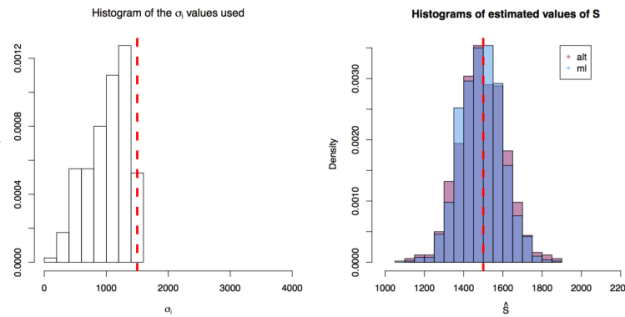 First simulation scenario where
  are shown by the blue (maximum likelihood) and red (alternative) histograms.
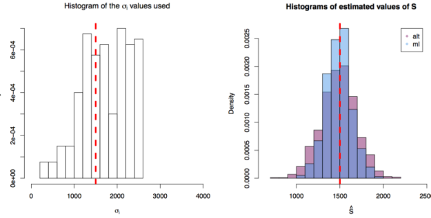 First simulation scenario where
  First simulation scenario where


