Experimental errors are common at the moment of generating new data. Often this type of errors are simply due to the inability of the instrument to make precise measurements. In addition, different instruments can have different levels of precision, even-thought they are used to perform the same measurement. Take for example two balances and an object with a mass of 1kg. The first balance, when measuring this object different times might record values of 1.0083 and 1.0091, and the second balance might give values of 1.1074 and 0.9828. In this case the first balance has a higher precision as the difference between its measurements is smaller than the difference between the measurements of balance two.
In order to have some control over this error introduced by the level of precision of the different instruments, they are labelled with a measure of their precision  or equivalently with their dispersion
  .
.
Let’s assume that the type of information these instruments record is of the form  , where
  is an error term,
  its the value recorded by instrument
  and where
  is the fixed true quantity of interest the instrument is trying to measure. But, what if is not a fixed quantity? or what if the underlying phenomenon that is being measured is also stochastic like the measurement . For example if we are measuring the weight of cattle at different times, or the length of a bacterial cell, or concentration of a given drug in an organism, in addition to the error that arises from the instruments; there is also some noise introduced by dynamical changes of the object that is being measured. In this scenario, the phenomenon of interest, can be given by a random variable
  . Therefore the instruments would record quantities of the form
  .
.
Under this case, estimating the value of  , the expected state of the phenomenon of interest is not a big challenge. Assume that there are
  values observed from realisations of the variables
  , which came from
  different instruments. Here
  is still a good estimation of as
  . Now, a more challenging problem is to infer what is the underlying variability of the phenomenon of interest
  . Under our previous setup, the problem is reduced to estimating
  as we are assuming and that the instruments record values of the from .
To estimate a standard maximum likelihood approach could be used, by considering the likelihood function:
 ,
,
from which the maximum likelihood estimator of is given by the solution to
![\sum [(X_i- \mu)^2 - (\sigma_i^2 + S^2)] /(\sigma_i^2 + S^2)^2 = 0](https://s0.wp.com/latex.php?latex=%5Csum+%5B%28X_i-+%5Cmu%29%5E2+-+%28%5Csigma_i%5E2+%2B+S%5E2%29%5D+%2F%28%5Csigma_i%5E2+%2B+S%5E2%29%5E2+%3D+0&bg=ffffff&fg=000&s=0&c=20201002) .
.
Another more naive approach could use the following result
![E[\sum (X_i-\sum X_i/n)^2] = (1-1/n) \sum \sigma_i^2 + (n-1) S^2](https://s0.wp.com/latex.php?latex=E%5B%5Csum+%28X_i-%5Csum+X_i%2Fn%29%5E2%5D+%3D+%281-1%2Fn%29+%5Csum+%5Csigma_i%5E2+%2B+%28n-1%29+S%5E2&bg=ffffff&fg=000&s=0&c=20201002)
from which  .
.
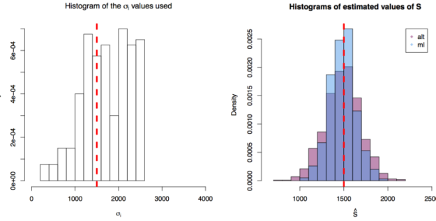
Here are three simulation scenarios where 200 values are taken from instruments of varying precision or variance  and where the variance of the phenomenon of interest
  . In the first scenario are drawn from
 ![[10,1500^2]](https://s0.wp.com/latex.php?latex=%5B10%2C1500%5E2%5D&bg=ffffff&fg=000&s=0&c=20201002) , in the second from
, in the second from ![[10,1500^2 \times 3]](https://s0.wp.com/latex.php?latex=%5B10%2C1500%5E2+%5Ctimes+3%5D&bg=ffffff&fg=000&s=0&c=20201002) and in the third from
and in the third from ![[10,1500^2 \times 5]](https://s0.wp.com/latex.php?latex=%5B10%2C1500%5E2+%5Ctimes+5%5D&bg=ffffff&fg=000&s=0&c=20201002) . In each scenario the value of
. In each scenario the value of  is estimated 1000 times taking each time another 200 realisations of . The values estimated via the maximum likelihood approach are plotted in blue, and the values obtained by the alternative method are plotted in red. The true value of the is given by the red dashed line across all plots.
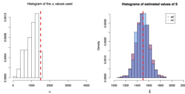 First simulation scenario where in . The values of plotted in the histogram to the right. The 1000 estimations of
  are shown by the blue (maximum likelihood) and red (alternative) histograms.
 First simulation scenario where in . The values of plotted in the histogram to the right. The 1000 estimations of are shown by the blue (maximum likelihood) and red (alternative) histograms.
 First simulation scenario where in . The values of plotted in the histogram to the right. The 1000 estimations of are shown by the blue (maximum likelihood) and red (alternative) histograms.
For recent advances in methods that deal with this kind of problems, you can look at:
Delaigle, A. and Hall, P. (2016), Methodology for non-parametric deconvolution when the error distribution is unknown. Journal of the Royal Statistical Society: Series B (Statistical Methodology), 78: 231–252. doi: 10.1111/rssb.12109


