Covariate Shift in Virtual Screening

In supervised learning, we assume that the training data and testing are drawn from the same distribution, i.e P_{train}(x,y) = P_{test}(x,y). However this assumption is often violated in virtual screening. For example, a chemist initially focuses on a series of compounds and the information from this series is used to train a model. For some reasons,  the chemist changes their focus on a new, structurally distinct series later on and we would not expect the model to accurately predict the labels in the testing sets.  Here, we introduce some methods to address this problem.

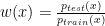
Methods such as Kernel Mean Matching (KMM) or Kullback-Leibler Importance Estimation Procedure (KLIEP) have been proposed.  These methods typically assume the concept remain unchanged and only the distribution changes, i.e. P_{train}(y|x) =P_{test}(y|x) and P_{train}(x) \neq P_{test}(x).  In general, these methods  reweight instances in the training data so that the distribution of training instances is more closely aligned with the distribution of instances in the testing set. The appropriate importance weighting factor w(x) for each instance x in the training set is:

w(x) = \frac{p_{test}(x)}{p_{train}(x)}

where p_{train}(x) is the training set density and p_{test} (x) is the testing set density. Note that only the feature vector values (not their labels) are used in reweighting. The major difference between KMM and KLIEP is the objective function: KLIEP is based on the minimisation of the Kullback-Leibler divergence while KMM is based on the minimisation of Maximum Mean Discrepancy (MMD).  For more detail, please see reference.

Reference:

  1. Masashi Sugiyama ,Taiji Suzuki, Shinichi Nakajima, Hisashi Kashima, Paul von Bünau, Motoaki Kawanabe.: Direct importance estimation for Covariate Shift Adaptation. Ann Inst Stat Math. 2008
  2. Jiayuan Huang,  Alex Smola, Arthur Gretton, Karsten Borgwardt, Bernhard Scholkopf.:Correcting Sample Selection Bias by Unlabeled Data. NIPS 06.
  3. Mcgaughey, Georgia ; Walters, W Patrick ; Goldman, Brian.: Understanding covariate shift in model performance. F1000Research, 2016,


Protein Engineering and Structure Determination

Sometimes it can be advantageous to combine two proteins into one. One such technique was described by Jennifer Padilla, Christos Colovos, and Todd Yeates back in 2001 (Padilla, et al., 2001). By connecting two proteins, one that dimerized, and another that trimerized, they were able to design synthetic ‘nanohedra’. The way they achieved this was by extending a C-terminal α-helix at the end of one protein by another α-helix ‘linker’, directly into the N-terminal α-helix of another protein:

Continue reading →

Introduction to R Markdown

Two of our esteemed OPIGlets presented a workshop on collaborative research using Jupyter Notebook this week at ISMB in Chicago. Their workshop highlights the importance of finding ways to share your work conveniently and reproducibly. So on a related note, I thought I would share a brief introduction to another useful tool, R Markdown with RStudio, which I use to present updates to various supervisors and to remember what I did three months (or three days) ago. This method of sharing work is highly readable, reproducible, and narrative-driven.

I use R for much of my data analysis and all of my visualisation, and I count the tidyverse among my most beloved friends. If you’re so inclined, it’s easy to execute python, bash, and more from within R Markdown. You also don’t need to use RStudio to use R Markdown, but that’s a whole other story.

Starting a new markdown file in RStudio will generate a template script explaining most of what you need to know. If I showed you that then I’d be out of a blog post, but I will at least link to the R Markdown Reference Guide.

R Markdown files consist of text written in markdown, and code chunks that can be individually executed and displayed inline within RStudio. To “knit” the whole thing together, the knitr package is used to execute and combine code chunks, then pandoc converts the whole thing into an attractive document.

Here’s an example. The metadata at the top sets up the document. I’ll be generating an html document here, but notice some other tempting examples commented out. Yes, you can use it for Latex (swoon). You can even make a Word document, but really, why would you?

---
title: "Informative Title"
author: "Clare E. West"
date: "10/07/2018"
output: html_document
#output: beamer_presentation
#output: pdf_document
---

```{r setup, include=FALSE}
knitr::opts_chunk$set(echo = TRUE)
library(knitr)
library(ggplot2)
library(tidyr)
library(dplyr)
```

## Big Title
### Smaller title

R Markdown scripts have the extension .Rmd

R Markdown is __so__ *fun*. You can read all about it [here](https://www.rstudio.com/wp-content/uploads/2015/03/rmarkdown-reference.pdf).

```{r}
print("Hello world")
```

Notice that chunks are enclosed within three backticks, with the language and options in braces. Single commands can be executed inline using single backticks.

As highlighted in the example above, global options are set like this:

knitr::opts_chunk$set(echo = TRUE)

“echo=TRUE” means that the code in each chunk is displayed in the final product; this is useful to show collaborators (or your future self) exactly how you did something. Change this option (“echo = FALSE”) globally or in individual blocks to prevent code from printing. This is useful to hide uninteresting commands, or when presenting to people who don’t have the time or inclination to read your code (hard to imagine). Notice I’ve also used “include = FALSE”  for the library-loading code chunk, which means evaluate but don’t include in the output. Another useful option is “eval = FALSE”, which means don’t even run this chunk.

So let’s see what that looks like when we render it:

The above example output as HTML

The above example output as Latex

Plots generated in code chunks or images from other sources can be embedded. Set the width in the options. “fig.width” sets the width (in inches) of the figure generated, while “out.width” scales the image in the final documents, for which the units will depend on the document type. Within RStudio, these are previewed inline below the code chunk.

## Including plots/images
```{r fig.width = 4, fig.height = 3, out.width = "400px", echo=FALSE}
t  %>% group_by(Tour, Winner, N, Tournament) %>% filter(WRank <= 20) %>% summarise(WPts = max(WPts))  %>% ggplot(aes(x=N, y=WPts, group=Winner, colour=(Winner=="Murray A."))) + geom_point() + geom_line() + labs(x="Tournament Number",y="Ranking Points") + scale_colour_discrete("",labels=c("Not Andy Murray", "Andy Murray")) + theme_bw() + theme(legend.position = "bottom", legend.margin = margin(0, 0, 0, 0))
knitr::include_graphics("https://s.yimg.com/ny/api/res/1.2/69ZUzNSMYb09GKd8CNJeew--~A/YXBwaWQ9aGlnaGxhbmRlcjtzbT0xO3c9ODAwO2g9NjAw/http://media.zenfs.com/en_us/News/afp.com/0102e1f7d0d3c35303c8a62d56a5eb79c2c8b4d8.jpg")
```

Rather than just printing data R-style, you can nicely format it into a table using kable (part of knitr). I also style mine using kableExtra, which makes it look nice and gives you extra options. By default tables fill the full width, you can override this using e.g. kable_styling(full.width = FALSE, position = “left”). When making a latex document, use kable(table, booktabs = T, “latex”) to get a (reproducible) latex-style table.

Here’s how to use python and bash. Thanks to the package reticulate, you can even share objects between your R and Python chunks. Exclude reticulate (knitr::opts_chunk$set(python.reticulate=FALSE) if you prefer to keep your languages separate.


### Mix it up with python
```{python}
a='Wow python'
print(a.split()[0])
```

What a wild ride. 

### or bash

```{bash, echo=TRUE}
ls | head 
```

Oh look, there's our output, ready to share.

Finally, if you hate GUIs – and you know I do – you can ditch the interactive notebook part and just generate documents from R Markdown files like this:

rmarkdown::render("BlogExample.Rmd")


Maps are useful. But first, you need to build, store and read a map.

Recently we embarked on a project that required the storage of a relatively big dictionary with 10M+ key-value pairs. Unsurprisingly, Python took over two hours to build such dictionary, taking into accounts all the time for extending, accessing and writing to the dictionary, AND it eventually crashed. So I turned to C++ for help.

In C++, map is one of the ways you can store a string-key and an integer value. Since we are concerned about the data storage and access, I compared map and unordered_map.

An unordered_map stores a hash table of the keys and the mapped value; while a map is ordered. The important consideration here includes:
  • Memory: map does not have the hash table and is therefore smaller than an unordered_map.
  • Access: accessing an unordered_map takes O(1) while accessing a map takes log(n).
I have eventually chosen to go with map, because it is more memory efficient considering the small RAM size that I have access to. However, it still takes up about 8GB of RAM per object during its runtime (and I have 1800 objects to run through, each building a different dictionary). Saving these seems to open another can of worm.
In Python, we could easily use Pickle or JSON to serialise the dictionary. In C++, it’s common to use the BOOST library. There are two archival functions in BOOST: text or binary archives. Text archives are human-readable but I don’t think I am really going to open and read 10M+ lines of key-value pairs, I opted for binary archives that are machine readable and smaller. (Read more: https://stackoverflow.com/questions/1058051/boost-serialization-performance-text-vs-binary-format .)
To further compress the memory size when I save the maps, I used zlib compression. Obviously there are ready-to-use codes from these people half a year ago, which saved me debugging:
Ultimately this gets down to 96GB summing 1800 files, all done within 6 hours.

Le Tour de Farce v6.0

Tuesday the 12th of June brought sun, cycling and beer to the land of OPIG. It was once again time for the annual Tour de Farce.

Le tour, now in its highly refined 6.0 version, covered a route which took us from the statistics department at Oxford (home to many OPIGlets) to our first port of call, The Head of the River pub. We then followed the river Isis (or Thames if you prefer) from the head of the river towards Osney mead.

Passing though Osney we soon arrived at our second waypoint. The Punter. One of the OPIGlets lived locally and so we were met by their trusty companion, who was better behaved than many of the others on Le Tour.

Departing the punter on two wheels (or in one case, on one) we followed the river upstream to The Perch.


Our arrival at The Perch was slightly hampered by a certain OPIGlet taking out anything in her path in her excitement.  Mr Sulu.. Ramming speed.


Those that survived soon left the perch, as we were once again headed upstream, this time to The Trout.

Having braved about half the journey it was now time for another restorative beverage and to take on supplies.  Sustenance was provided by Jacob’s Inn.   Jacob’s Inn has the advantage of goats, chickens and pigs in the back garden.  Having spent most of the afternoon in each other’s company, the company of pigs was preferable for some.

As we finished dinner, the sun was beginning to set and so we abandoned the original plan of finishing off at The Fishes.  Instead we returned southwards where we closed off the evening with a drink at The Royal Oak, mere yards from where we started the day.

The route of the 2018 v6.0 Tour de Farce.


Storing your stuff with clever filesystems: ZFS and tmpfs

The filesystem is a a critical component of just about any operating system, however it’s often overlooked. When setting up a new server, the default filesystem options are often ticked and never thought about again. However, there exist a couple of filesystems which can provide some extraordinary features and speed. I’m talking about ZFS and tmpfs.

ZFS was originally developed by Oracle for their Solaris operating system, but has now been open-sourced and is freely available on linux. Tmpfs is a temporary file system which uses system memory to provide fast temporary storage for files. Together, they can provide outstanding reliability and speed for not very much effort.

Hard disk capacity has increased exponentially over the last 50 years. In the 1960s, you could rent a 5MB hard disk from IBM for the equivalent of $130,000 per month. Today you can buy for less than $600 a 12TB disk – a 2,400,000 times increase.

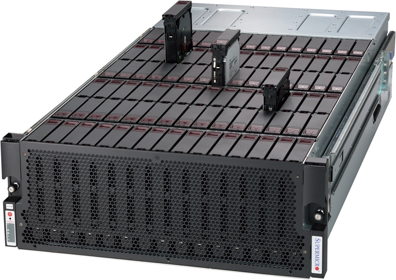
As storage technology has moved on, the filesystems which sit on top of them ideally need to be able to access the full capacity of those ever increasing disks. Many relatively new, or at least in-use, filesystems have serious limitations. Akin to “640K ought to be enough for anybody”, the likes of the FAT32 filesystem supports files which are at most 4GB on a chunk of disk (a partition) which can be at most 16TB. Bear in mind that arrays of disks can provide a working capacity of many times that of a single disk. You can buy the likes of a supermicro sc946ed shelf which will add 90 disks to your server. In an ideal world, as you buy bigger disks you should be able to pile them into your computer and tell your existing filesystem to make use of them, your filesystem should grow and you won’t have to remember a different drive letter or path depending on the hardware you’re using.

ZFS is a 128-bit file system, which means a single installation maxes out at 256 quadrillion zettabytes. All metadata is allocated dynamically so there isn’t the need to pre-allocate inodes and directories can have up to 2^48 (256 trillion) entries. ZFS provides the concept of “vdevs” (virtual devices) which can be a single disk or redundant/striped collections of multiple disks. These can be dynamically added to a pool of vdevs of the same type and your storage will grow onto the fresh hardware.

A further consideration is that both disks of the “spinning rust” variety and SSDs are subject to silent data corruption, i.e. “bit rot”. This can be caused by a number of factors even including cosmic rays, but the consequence is read errors when it comes time to retrieve your data. Manufacturers are aware of this and buried in the small print for your hard disk will be values for “unrecoverable read errors” i.e. data loss. ZFS works around this by providing several mechanisms:

  • Checksums for each block of data written.
  • Checksums for each pointer to data.
  • Scrub – Automatically validates checksums when the system is idle.
  • Multiple copies – Even if you have a single disk, it’s possible to provide redundancy by setting a copies=n variable during filesystem creation.
  • Self-healing – When a bad data block is detected, ZFS fetches the correct data from a redundant copy and replaces it with the correct data.

An additional bonus to ZFS is its ability to de-duplicate data. Should you be working with a number of very similar files, on a normal filesystem, each file will take up space proportional to the amount of data that’s contained. As ZFS keeps checksums of each block of data, it’s able to determine if two blocks contain identical data. ZFS therefore provides the ability to have multiple pointers to the same file and only store the differences between them.


ZFS also provides the ability to take a point in time snapshot of the entire filesystem and roll it back to a previous time. If you’re a software developer, got a package that has 101 dependencies and you need to upgrade it? Afraid to upgrade it in case it breaks things horribly? Working on code and you want to roll back to a previous version? ZFS snapshots can be run with cron or manually and provide a version of the filesystem which can be used to extract previous versions of overwritten or deleted files or used to roll everything back to a point in time when it worked.

Similar to deduplication, a snapshot won’t take up any disk extra space until the data starts to change.

The other filesystem worth mentioning is tmpfs. Tmpfs takes part of the system memory and turns it into a usable filesystem. This is incredibly useful for systems which create huge numbers of temporary files and attempt to re-read them. Tmpfs is also just about as fast as a filesystem can be. Compared to a single SSD or a RAID array of six disks, tmpfs blows them out of the water speed wise.

Creating a tmpfs filesystem is simple:
First create your mountpoint for the disk:

mkdir /mnt/ramdisk

Then mount it. The options are saying make it 1GB in size, it’s of type tmpfs and to mount it at the previously created mount point:

mount –t tmpfs -o size=1024m tmpfs /mnt/ramdisk

At this point, you can use it like any other filesystem:

df -h
Filesystem Size Used Avail Use% Mounted on
/dev/sda1  218G 128G   80G  62% /
/dev/sdb1  6.3T 2.4T  3.6T  40% /spinnyrust
tank       946G 3.5G  942G   1% /tank
tmpfs      1.0G 391M  634M  39% /mnt/ramdisk

OPIG at the Oxford Maths Festival

Men with glasses poring over long columns of numbers. Tabulation of averages and creation of data tables. Lots of counting. The public image of statistics hardly corresponds to what OPIG do – even where OPIG’s work is at its most formally statistical.

OPIG exhibited a street stall at the Oxford Maths Festival to try to change that perception. How do you interest passers-by in real statistics without condescending and without oversimplifying? Data is becoming more important in the lives of all kinds of people and we need to be clear that it isn’t magic, but neither is it trivial. We need to prove that the kind of thoughtful reasoning that people put into managing their lives is the same kind of thing we do in data analysis.

Let’s look at one activity that OPIG did on the street at the Oxford Maths Festival.

The idea

We started with a compelling story: rumors were flying during the Second World War about how many tanks the Germans were producing. Allied intelligence needed to figure out if these numbers were true. In its simple retelling, the Germans simply numbered their tanks, but in truth there were two sequences of gearbox numbers, complicated chassis and engine numbers, and a set of numbered wheel moulds which left numbers imprinted in each of the wheels of the tanks.

However you parse it, the relevant problem is finding out how many gearboxes, chassis, wheels, or engines were in use, which tells you how many tanks are being produced, since no tank can have, for example, more than one engine. It’s a little hard to get close to a German tank, so Allied soldiers collected these numbers when they were destroyed.

This problem – finding the largest number of a range 1, 2, 3, 4, … N – is known generally as the German Tank Problem. Most mathematics educators have some familiarity with it, but on the street we found it works really well. This observation presumably speaks to the paucity of mathematics educators on the street.

How it works

The demonstration, while straightforward and quick, has a few subtleties. We cut open a box and cut 4750 slips of paper, numbered from 1 to 4750.

The first step is to ask how many slips of paper are in the box. Answers varied from one hundred to more than 10,000. Shaking the box helped encourage unreliable guesses and prevented people from reading the numbers off the slips in the box.

Then we asked people to pick one piece of paper out of the box and update their guess. We found a few aspects of this to be interesting. It is trivial to convince people that they will not get the top number in their guess. We all, then, have an intuition that the number drawn at this stage should be ‘somewhere in the middle’, which is completely wrong. There’s no particular reason to think that the guess should be in any interval over the distribution. It is true, however, that the mean of the first number chosen after many runs of the demonstration is 2375 and reasoning about average behaviour in this way turns out to be very powerful.

We then would ask people to draw up to four more slips. The point that people should absorb at this stage is that those guesses should assort evenly over the possible distribution, and you only need to add ‘a little bit more’ to compensate for this effect. We then precomputed the best guess for various numbers because the calculation is too tedious for a streetcorner – from which it becomes obvious that having more than five slips is nearly unnecessary to guess the maximum well. (See the histogram of estimates from five-slip draws below.) And 60% of guesses were slightly high of the true number, but the guesses that were too low tended to be much too low.

Going from blind indifference to a really solid guess is a powerful experience, and we can take people through it with every step of the reasoning on display. It shows what data analysis looks like at the research level and can be a great experience for the public.

How to parse OAS data

We have recently released the Observed Antibody Space database – collection of cleaned and annotated antibody sequence (Ig-seq or AIRR-seq) data from 53 studies. We have formatted the data in the format that should facilitate data mining and since release we had several queries on how to parse the data out. Therefore here we give a small example of how to parse the data and make sense of it.

You should download the bulk data file from OAS, available here.

The datasets are separated into ‘data units‘  – collections of sequences that can be uniquely assigned to a range of metadata parameters such as study, organism etc. Our task therefore is to iterate through all those files and read sequences from each of these. Firstly we will attempt to iterate through the files and I will assume that you uncompressed the bulk data file into ../data/json folder. We will write a helper function that will simply list all files with its full paths in a directory and call it list_file_paths

import os

#Fetch all files in directory and subdirectories.
def list_file_paths(directory):
   for dirpath,_,filenames in os.walk(directory):
       for f in filenames:
           yield os.path.abspath(os.path.join(dirpath, f))

if __name__ == '__main__':
    #Replace this with the location of where you uncompressed the bulk data file.
    directory = '../data/json'

    for f in list_file_paths(directory):
        print f

The code above will list all the files in ../data/json which incidentally are all the ‘data units’. Now our task is to parse out the output from each of the data units. They are gzipped files with data element on each line. Therefore we will use gzip library to stream the contents of a gzipped file rather than uncompressing each one of them separately. This is achieved by function parse_single_file

import os,gzip

#Fetch all files in directory and subdirectories.
def list_file_paths(directory):
   for dirpath,_,filenames in os.walk(directory):
       for f in filenames:
           yield os.path.abspath(os.path.join(dirpath, f))

#Parse out the contents of a single file.
def parse_single_file(src):
    #The first line are the meta entries.
    meta_line = True
    for line in gzip.open(src,'rb'):
        print line
    

if __name__ == '__main__':
    #Replace this with the location of where you uncompressed the bulk data file.
    directory = '../data/json'

    for f in list_file_paths(directory):
        parse_single_file(f)

The code above will simply go through all the data unit files, stream the gzipped lines and print each one of them separately. Each line however is formatted as json – meaning it can be parsed using pythons json library and act as a pythonic dictionary. below we have parsed out the basic elements in the final incarnation of the code:

import os,gzip,json,pprint

#Fetch all files in directory and subdirectories.
def list_file_paths(directory):
   for dirpath,_,filenames in os.walk(directory):
       for f in filenames:
           yield os.path.abspath(os.path.join(dirpath, f))

#Parse out the contents of a single file.
def parse_single_file(src):
    #The first line are the meta entries.
    meta_line = True
    for line in gzip.open(src,'rb'):
        if meta_line == True:
                metadata = json.loads(line)
                meta_line=False
                print "Metadata:"
                pprint.pprint(metadata)
                continue
        #Parse actual sequence data.
        basic_data = json.loads(line)
        print "Basic data:"
        pprint.pprint(basic_data)

        #IMGT-Numbered sequence.
        print "IMGT-numbered sequence"
        d = json.loads(basic_data['data'])
        pprint.pprint(d)
        print "==========="
    
if __name__ == '__main__':
    #Replace this with the location of where you uncompressed the bulk data file.
    directory = '../data/json'

    for f in list_file_paths(directory):
        parse_single_file(f)

The first line of each data unit are meta entries. These look as follows:

{u'Age': u'22-70',
 u'Author': u'Halliley et al., (2015)',
 u'BSource': u'Bone-Marrow',
 u'BType': u'Plasma-B-Cells',
 u'Chain': u'Heavy',
 u'Disease': u'None',
 u'Isotype': u'IGHM',
 u'Link': u'https://doi.org/10.1016/j.immuni.2015.06.016',
 u'Longitudinal': u'no',
 u'Size': 934,
 u'Species': u'human',
 u'Subject': u'no',
 u'Vaccine': u'Tetanus/Flu'}

The attributes should be self-explanatory and the existence of this data on top of each file is supposed to streamline searching through data-units if you wish to parse sequences given a particular configuration of meta-data entries (e.g. organism).

Next, the code parses out data on each sequence that is associated with its genes, full sequence, CDR3 and numbered sequence. Therefore the output for this will look something like this:

{u'cdr3': u'ARHQGVYWVTTAGLSH',
 u'data': u'{"fwh1": {"11": "G", "24": "T", "13": "V", "12": "L", "15": "P", "14": "K", "17": "E", "16": "S", "19": "L", "18": "T", "22": "T", "26": "S", "25": "V", "21": "L", "20": "S", "23": "C"}, "fwh3": {"68": "N", "88": "S", "89": "L", "66": "Y", "67": "Y", "82": "T", "83": "S", "80": "V", "81": "D", "86": "Q", "87": "F", "84": "K", "85": "N", "92": "S", "79": "S", "69": "P", "104": "C", "78": "I", "77": "T", "76": "V", "75": "R", "74": "S", "72": "K", "71": "L", "70": "S", "102": "Y", "90": "K", "100": "A", "101": "V", "95": "T", "94": "V", "97": "A", "96": "A", "91": "L", "99": "T", "98": "D", "93": "S", "103": "Y"}, "fwh2": {"52": "W", "39": "W", "48": "Q", "49": "G", "46": "P", "47": "G", "44": "Q", "45": "P", "51": "E", "43": "R", "40": "G", "42": "I", "55": "S", "53": "I", "54": "G", "41": "W", "50": "L"}, "fwh4": {"120": "Q", "121": "G", "122": "T", "123": "L", "124": "V", "125": "P", "126": "V", "127": "S", "128": "S", "119": "G", "118": "W"}, "cdrh1": {"27": "G", "37": "Y", "31": "S", "30": "I", "28": "G", "29": "S", "35": "S", "34": "S", "38": "Y", "36": "S"}, "cdrh2": {"59": "S", "58": "Y", "57": "S", "56": "I", "63": "G", "64": "T", "65": "T"}, "cdrh3": {"111A": "W", "109": "G", "108": "Q", "115": "L", "114": "G", "117": "H", "116": "S", "111": "Y", "110": "V", "113": "A", "112": "T", "112A": "T", "112B": "V", "106": "R", "107": "H", "105": "A"}}',
 u'j': u'IGHJ1*01',
 u'name': 12,
 u'redundancy': 1,
 u'seq': u'GLVKPSETLSLTCTVSGGSISSSSYYWGWIRQPPGQGLEWIGSISYSGTTYYNPSLKSRVTISVDTSKNQFSLKLSSVTAADTAVYYCARHQGVYWVTTAGLSHWGQGTLVPVSS',
 u'v': u'IGHV4-39*07'}

Above, redundancy refers to how many times we see a given sequence (seq) in a particular study. We also store the IMGT-numbered data (the data attribute) which needs a second round of json parsing and its output is a dictionary of IMGT-number – amino acid associations grouped by the regions of an antibody (cdrs and framework regions):

{u'cdrh1': {u'27': u'G',
            u'28': u'G',
            u'29': u'S',
            u'30': u'I',
            u'31': u'S',
            u'34': u'S',
            u'35': u'S',
            u'36': u'S',
            u'37': u'Y',
            u'38': u'Y'},
 u'cdrh2': {u'56': u'I',
            u'57': u'S',
            u'58': u'Y',
            u'59': u'S',
            u'63': u'G',
            u'64': u'T',
            u'65': u'T'},
 u'cdrh3': {u'105': u'A',
            u'106': u'R',
            u'107': u'H',
            u'108': u'Q',
            u'109': u'G',
            u'110': u'V',
            u'111': u'Y',
            u'111A': u'W',
            u'112': u'T',
            u'112A': u'T',
            u'112B': u'V',
            u'113': u'A',
            u'114': u'G',
            u'115': u'L',
            u'116': u'S',
            u'117': u'H'},
 u'fwh1': {u'11': u'G',
           u'12': u'L',
           u'13': u'V',
           u'14': u'K',
           u'15': u'P',
           u'16': u'S',
           u'17': u'E',
           u'18': u'T',
           u'19': u'L',
           u'20': u'S',
           u'21': u'L',
           u'22': u'T',
           u'23': u'C',
           u'24': u'T',
           u'25': u'V',
           u'26': u'S'},
 u'fwh2': {u'39': u'W',
           u'40': u'G',
           u'41': u'W',
           u'42': u'I',
           u'43': u'R',
           u'44': u'Q',
           u'45': u'P',
           u'46': u'P',
           u'47': u'G',
           u'48': u'Q',
           u'49': u'G',
           u'50': u'L',
           u'51': u'E',
           u'52': u'W',
           u'53': u'I',
           u'54': u'G',
           u'55': u'S'},
 u'fwh3': {u'100': u'A',
           u'101': u'V',
           u'102': u'Y',
           u'103': u'Y',
           u'104': u'C',
           u'66': u'Y',
           u'67': u'Y',
           u'68': u'N',
           u'69': u'P',
           u'70': u'S',
           u'71': u'L',
           u'72': u'K',
           u'74': u'S',
           u'75': u'R',
           u'76': u'V',
           u'77': u'T',
           u'78': u'I',
           u'79': u'S',
           u'80': u'V',
           u'81': u'D',
           u'82': u'T',
           u'83': u'S',
           u'84': u'K',
           u'85': u'N',
           u'86': u'Q',
           u'87': u'F',
           u'88': u'S',
           u'89': u'L',
           u'90': u'K',
           u'91': u'L',
           u'92': u'S',
           u'93': u'S',
           u'94': u'V',
           u'95': u'T',
           u'96': u'A',
           u'97': u'A',
           u'98': u'D',
           u'99': u'T'},
 u'fwh4': {u'118': u'W',
           u'119': u'G',
           u'120': u'Q',
           u'121': u'G',
           u'122': u'T',
           u'123': u'L',
           u'124': u'V',
           u'125': u'P',
           u'126': u'V',
           u'127': u'S',
           u'128': u'S'}}

We hope this quick intro to our data format will allow you to do great science with this data.

Prague Protein Spring 2018

We, Constantin and Dominik, the newest members of OPIG (SABS rotation students, as usual) were lucky to have a conference suitable to our research within our rotation period and, granted an allowance from the powers that be, were able to visit this year’s Prague Protein Spring with the topic ‘Proteins at Work’. There, we spent four busy but very inspirational days with about 50 participants in a little palace, the Vila Lanna.

The general topic of this meeting led to a broad variety of talks representing a multitude of fields of protein research: from origins of life, over fuzzy intrinsically disordered proteins and crowded cells to metagenomics and functional sequence alignment annotation.

We picked four thought engaging talks to present at the group meeting on 08/05/2018; here are their summaries:

Protein engineering and in vitro evolution studies for the origins of life

Kosuke Fujishima from Tokyo Institute of Technology presented several examples of the research he conducts in the area of origins of life. Research on the origins of life are generally based around the questions how prebiotic monomers were created, how they condensed into polymers and how functionality emerged within these polymers.

The first example of his research deals with the condensation of prebiotic monomers on the ocean-earth crust-interface. Water cycling between the ocean and the outer layers of the earth’s core provided an environment of high pressure and high temperatures (80 – 200 °C) which is necessary for amino acid polymerisation. The mineral Olivine was found to attract amino acids to its surface and the serpentinisation reaction happening with Olivine might provide the necessary wet/dry cycle. Therefore, the researchers built a reactor aiming to investigate this potential polymerisation mechanism. They found that with providing six prebiotic amino acids, 28 out of 36 possible dipeptides could be found in the reactor. Furthermore, up to 10-mer linear polypeptides could be detected as well, providing evidence for a mechanism of early earth’s generation of polypeptides [unpublished].

The second project showed that both enzymes, CysE/CysK, responsible for the current production of cysteine from serine, could be re-engineered to contain no cysteine in their sequence. Interestingly, cysteine-free CysE showed higher reaction rates than the wild type. Additional reduction to cysteine- and methionine-free enzyme sequences only worked for CysE but not for CysK.[Fujishima et al. (2018)] Still, the experiments indicate that an enzyme world could have existed with a reduced number of amino acids compared to the 20(+) amino acids that we know today.

The third project we wanted to point out used a type of mRNA display that not only links the genotype (mRNA) with its corresponding phenotype (translated protein) but also allows the translated protein to interact with a randomised, non-translated part of the mRNA. This provided a framework for investigating the evolution of ribonucleotide-binding (RNP) proteins. When selecting for ATP-binding, it was observed that protein together with RNA had the best fitness landscape compared to protein selection or RNA selection alone. Further analysis revealed that most binding affinity of the ribonucleotide protein stemmed from its RNA part.[unpublished] These results give rise to the suggestion that RNA and proteins co-evolved, opposing the idea of a pure RNA world.

RNA-protein interactions and the structure of the genetic code

The next speaker added more to the research area of RNA-protein interaction and evolution. Bojan Zagrovic from the University of Vienna presented his research around the finding that pyrimidine (PYR) density of RNA regions is correlated with the corresponding protein region’s affinity to pyrimidine-containing bases (running means of 21 amino acids or 63 bases were used), with the highest correlation between mRNA PYR density and guanine affinity, having an average ‘typical’ Pearson correlation coefficient of 0.80.[Polyansky & Zagrovic (2013)]

This correlation is specific for the current genetic code, shown by random generation of genetic codes which could not reproduce such a correlated behaviour and by looking into three organisms with very different codon usage bias (homo sapiens, E. coli, M. jannaschii). Even though the three averages of codon usage were very different, the highest correlating pairs of mRNA and cognate proteins clustered together, having very similar codon usage. This was also true for the worst correlating pairs.[Hlevnjak & Zagrovic (2015)]

But the big question being: what does this correlation imply functionally?

Annotation analysis revealed that the highest correlating pairs were enriched in nucleotide-binding functions and intrinsically disordered proteins. Without claiming generalisability, Professor Zagrovic pointed out a case study done on RNA polymerase II which has a long disordered C-terminus build up by 26 repeats of a 7 amino acid motif. 248 RNAs were found to interact with RNA polymerase II and in all three reading frames of the interacting RNAs, amino acid codons of the polymerase’s C-terminus were enriched.[unpublished]

This indicates some regulation over gene expression but also several other hypotheses were made: the correlation between the protein regions’ affinity for their cognate mRNA regions might be relevant in virus assembly, since coding RNA and translated proteins have to be in close proximity with each other. The same could be true for some non-membrane-bound compartments, e.g. P-bodies. Or is this correlation characteristic a hint to mRNAs acting as chaperones for their respective proteins? The functional implications of this correlation, while highly speculative, nevertheless suggest exciting research to come in the future.

Fuzziness in protein assemblies

Research from a different, but equally thought provoking field was presented by Mónika Fuxreiter from the University of Debrecen. Her talk on the concept of fuzziness in protein complexes, which she introduced 10 years ago [Tompa & Fuxreiter (2008)], shed light on some more recent developments in the field as well as explaining the underlying concept for those of us (ourselves included) who have not encountered the concept as such before.

Fuzziness in the context of protein complexes describes a phenomenon in which intrinsically disordered proteins, instead of folding upon binding as one would usually observe, can sample several conformational states with different propensities, leading to the sampled states contributing with different strengths to the function of the protein complex and further leading to varying degrees of disorder in the bound state.

This observation has several implications for the understanding of the functionality of disordered proteins, since the relative propensity for different ensemble states in the bound form is thought to be highly susceptible to milieu influences, such as tissue specific splicing and post-translational modifications. Fuzziness (a term that was borrowed from the mathematical theory of fuzzy sets) could thus be a driver of functional adaptability of disordered proteins to cell-cycle stage, environmental influences or tissue type.

Evidence for fuzziness has been curated by the Fuxreiter group since 2015 [Miskei et al. 2017] in the FuzDB database and recently been used to develop a prediction algorithm [unpublished], that according to Professor Fuxreiter achieves highly accurate predictions of fuzziness on a comprehensive validation dataset.

Both the implications of fuzziness for the understanding of the mode of action for disordered proteins (and disordered regions in otherwise ordered proteins) certainly spiked our interest, not least due to the potential importance of a clear understanding of these mode of actions for drug development.

Investigation of mutually exclusive splicing events using the CATH FunFam framework

The last of the 4 talks we would like to single out in this blogpost highlighted recent progress in using structure-based databases for the investigation of complex cellular events.

Christine Orengo from UCL presented her group’s work on mutually exclusive splicing, which employed the FunFam framework of the CATH database to probe the structural and functional implications of these splicing events [Lam et al. (2018), under review].

The FunFams are a subcategory of CATH’s homologous superfamilies, which further divides the superfamilies based on clusters of residue conservation within each family, thus creating groupings of functionally related proteins [Rentzsch & Orengo (2013)].

Mutually exclusive splicing that were investigated using this framework are a group of splicing events in which only one of several specific exons is present in the spliced mRNA. These exons usually show a high level of sequence similarity, leading to a low disruption of the protein structure by the splicing event. It is thought that this feature is a reason for the relative enrichment of mutually exclusive exons amongst alternative splicing events in the proteome.

This high degree of sequence similarity further enabled the mapping of the mutually exclusive exons to FunFams in the CATH database and thus further onto protein structures. This allowed the Orengo group to conduct a ‘large scale systematic study of the structural/functional effects of MXE splicing’.

Their analysis found that variable residues between the exons are significantly enriched at the protein surface, both compared to other stretches of the protein sequence and compared to non-variable residues in the exons, and in close proximity (< 6 Angstroms) to functional sites of the protein.

The main conclusion drawn from these findings was that, as previously hypothesised, mutually exclusive exons are likely functional switches, since changes in the surface exposed area close to functional sites are likely to affect the protein function without strongly disrupting its structure.

In the eyes of the Orengo group, this makes these splicing events good candidates for drug targeting, particularly in cases where a tissue specific isoform can be drugged, since in that case off-target effects could potentially be significantly reduced.

Sources:

Fujishima et al. (2018). Reconstruction of cysteine biosynthesis using engineered cysteine-free enzymes. Scientific Reports

Hlevnjak & Zagrovic (2015). Malleable nature of mRNA-protein compositional complementarity and its functional significance. Nucleic Acids Res

Lam, S. D., Orengo, C., & Lees, J. (2018). Protein structure and function analyses to understand the implication of mutually exclusive splicing. BioRxiv

Miskei, M. et al (2017). FuzDB: Database of fuzzy complexes, a tool to develop stochastic structure-function relationships for protein complexes and higher-order assemblies. Nucleic Acids Research

Polyansky & Zagrovic (2013). Evidence of direct complementary interactions between messenger RNAs and their cognate proteins. Nucleic Acids Res

Rentzsch, R., & Orengo, C. A. (2013). Protein function prediction using domain families. BMC Bioinformatics

Tompa, P., & Fuxreiter, M. (2008). Fuzzy complexes: polymorphism and structural disorder in protein-protein interactions. Trends in Biochemical Sciences


Neuronal Complexity: A Little Goes a Long Way…To Clean My Apartment

The classical model of signal integration in both biological and Artificial Neural Networks looks something like this,

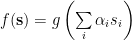
f(\mathbf{s})=g\left(\sum\limits_i\alpha_is_i\right)

where g is some linear or non-linear output function whose parameters \alpha_i adapt to feedback from the outside world through changes to protein dense structures near to the point of signal input, namely the Post Synaptic Density (PSD). In this simple model integration is implied to occur at the soma (cell body) where the input signals s_i are combined and broadcast to other neurons through downstream synapses via the axon. Generally speaking neurons (both artificial and otherwise) exist in multilayer networks composing the inputs of one neuron with the outputs of the others creating cross-linked chains of computation that have been shown to be universal in their ability to approximate any desired input-output behaviour.
See more at Khan Academy

Models of learning and memory have relied heavily on modifications to the PSD to explain modifications in behaviour. Physically these changes result from alterations in the concentration and density of the neurotransmitter receptors and ion channels that occur in abundance at the PSD, but, in actuality these channels occur all along the cell wall of the dendrite on which the PSD is located. Dendrites are something like a multi-branched mass of input connections belonging to each neuron. This begs the question as to whether learning might in fact occur all along the length of each densely branched dendritic tree.

Continue reading →