
Parsing command line arguments is an annoying piece of boilerplate we all have to do. Documenting our code is either an absolutely essential part of software engineering, or a frivolous waste of research time, depending on who you ask. But what if I told you that we can combine the two? That you can handle your argument parsing simply by documenting how your code works? Well, the dream is now reality. Continue reading
Category Archives: How To
Introduction to R Markdown
Two of our esteemed OPIGlets presented a workshop on collaborative research using Jupyter Notebook this week at ISMB in Chicago. Their workshop highlights the importance of finding ways to share your work conveniently and reproducibly. So on a related note, I thought I would share a brief introduction to another useful tool, R Markdown with RStudio, which I use to present updates to various supervisors and to remember what I did three months (or three days) ago. This method of sharing work is highly readable, reproducible, and narrative-driven.
I use R for much of my data analysis and all of my visualisation, and I count the tidyverse among my most beloved friends. If you’re so inclined, it’s easy to execute python, bash, and more from within R Markdown. You also don’t need to use RStudio to use R Markdown, but that’s a whole other story.
Starting a new markdown file in RStudio will generate a template script explaining most of what you need to know. If I showed you that then I’d be out of a blog post, but I will at least link to the R Markdown Reference Guide.
R Markdown files consist of text written in markdown, and code chunks that can be individually executed and displayed inline within RStudio. To “knit” the whole thing together, the knitr package is used to execute and combine code chunks, then pandoc converts the whole thing into an attractive document.
Here’s an example. The metadata at the top sets up the document. I’ll be generating an html document here, but notice some other tempting examples commented out. Yes, you can use it for Latex (swoon). You can even make a Word document, but really, why would you?
---
title: "Informative Title"
author: "Clare E. West"
date: "10/07/2018"
output: html_document
#output: beamer_presentation
#output: pdf_document
---

```{r setup, include=FALSE}
knitr::opts_chunk$set(echo = TRUE)
library(knitr)
library(ggplot2)
library(tidyr)
library(dplyr)
```

## Big Title
### Smaller title

R Markdown scripts have the extension .Rmd

R Markdown is __so__ *fun*. You can read all about it [here](https://www.rstudio.com/wp-content/uploads/2015/03/rmarkdown-reference.pdf).

```{r}
print("Hello world")
```
Notice that chunks are enclosed within three backticks, with the language and options in braces. Single commands can be executed inline using single backticks.
As highlighted in the example above, global options are set like this:
knitr::opts_chunk$set(echo = TRUE)
“echo=TRUE” means that the code in each chunk is displayed in the final product; this is useful to show collaborators (or your future self) exactly how you did something. Change this option (“echo = FALSE”) globally or in individual blocks to prevent code from printing. This is useful to hide uninteresting commands, or when presenting to people who don’t have the time or inclination to read your code (hard to imagine). Notice I’ve also used “include = FALSE” for the library-loading code chunk, which means evaluate but don’t include in the output. Another useful option is “eval = FALSE”, which means don’t even run this chunk.
So let’s see what that looks like when we render it:

The above example output as HTML

The above example output as Latex
Plots generated in code chunks or images from other sources can be embedded. Set the width in the options. “fig.width” sets the width (in inches) of the figure generated, while “out.width” scales the image in the final documents, for which the units will depend on the document type. Within RStudio, these are previewed inline below the code chunk.
## Including plots/images
```{r fig.width = 4, fig.height = 3, out.width = "400px", echo=FALSE}
t  %>% group_by(Tour, Winner, N, Tournament) %>% filter(WRank <= 20) %>% summarise(WPts = max(WPts))  %>% ggplot(aes(x=N, y=WPts, group=Winner, colour=(Winner=="Murray A."))) + geom_point() + geom_line() + labs(x="Tournament Number",y="Ranking Points") + scale_colour_discrete("",labels=c("Not Andy Murray", "Andy Murray")) + theme_bw() + theme(legend.position = "bottom", legend.margin = margin(0, 0, 0, 0))
knitr::include_graphics("https://s.yimg.com/ny/api/res/1.2/69ZUzNSMYb09GKd8CNJeew--~A/YXBwaWQ9aGlnaGxhbmRlcjtzbT0xO3c9ODAwO2g9NjAw/http://media.zenfs.com/en_us/News/afp.com/0102e1f7d0d3c35303c8a62d56a5eb79c2c8b4d8.jpg")
```

Rather than just printing data R-style, you can nicely format it into a table using kable (part of knitr). I also style mine using kableExtra, which makes it look nice and gives you extra options. By default tables fill the full width, you can override this using e.g. kable_styling(full.width = FALSE, position = “left”). When making a latex document, use kable(table, booktabs = T, “latex”) to get a (reproducible) latex-style table.

Here’s how to use python and bash. Thanks to the package reticulate, you can even share objects between your R and Python chunks. Exclude reticulate (knitr::opts_chunk$set(python.reticulate=FALSE) if you prefer to keep your languages separate.
### Mix it up with python
```{python}
a='Wow python'
print(a.split()[0])
```

What a wild ride.

### or bash

```{bash, echo=TRUE}
ls | head
```

Oh look, there's our output, ready to share.

Finally, if you hate GUIs – and you know I do – you can ditch the interactive notebook part and just generate documents from R Markdown files like this:
rmarkdown::render("BlogExample.Rmd")
Maps are useful. But first, you need to build, store and read a map.
Recently we embarked on a project that required the storage of a relatively big dictionary with 10M+ key-value pairs. Unsurprisingly, Python took over two hours to build such dictionary, taking into accounts all the time for extending, accessing and writing to the dictionary, AND it eventually crashed. So I turned to C++ for help.
In C++, map is one of the ways you can store a string-key and an integer value. Since we are concerned about the data storage and access, I compared map and unordered_map.
(Read more: https://www.geeksforgeeks.org/map-vs-unordered_map-c/ .)
An
unordered_map stores a hash table of the keys and the mapped value; while a map is ordered. The important consideration here includes:- Memory:
mapdoes not have the hash table and is therefore smaller than anunordered_map. - Access: accessing an
unordered_maptakes O(1) while accessing amaptakes log(n).
I have eventually chosen to go with
map, because it is more memory efficient considering the small RAM size that I have access to. However, it still takes up about 8GB of RAM per object during its runtime (and I have 1800 objects to run through, each building a different dictionary). Saving these seems to open another can of worm.In Python, we could easily use Pickle or JSON to serialise the dictionary. In C++, it’s common to use the BOOST library. There are two archival functions in BOOST: text or binary archives. Text archives are human-readable but I don’t think I am really going to open and read 10M+ lines of key-value pairs, I opted for binary archives that are machine readable and smaller. (Read more: https://stackoverflow.com/questions/1058051/boost-serialization-performance-text-vs-binary-format .)
To further compress the memory size when I save the maps, I used zlib compression. Obviously there are ready-to-use codes from these people half a year ago, which saved me debugging:
Ultimately this gets down to 96GB summing 1800 files, all done within 6 hours.
Storing your stuff with clever filesystems: ZFS and tmpfs
The filesystem is a a critical component of just about any operating system, however it’s often overlooked. When setting up a new server, the default filesystem options are often ticked and never thought about again. However, there exist a couple of filesystems which can provide some extraordinary features and speed. I’m talking about ZFS and tmpfs.
ZFS was originally developed by Oracle for their Solaris operating system, but has now been open-sourced and is freely available on linux. Tmpfs is a temporary file system which uses system memory to provide fast temporary storage for files. Together, they can provide outstanding reliability and speed for not very much effort.
Hard disk capacity has increased exponentially over the last 50 years. In the 1960s, you could rent a 5MB hard disk from IBM for the equivalent of $130,000 per month. Today you can buy for less than $600 a 12TB disk – a 2,400,000 times increase.

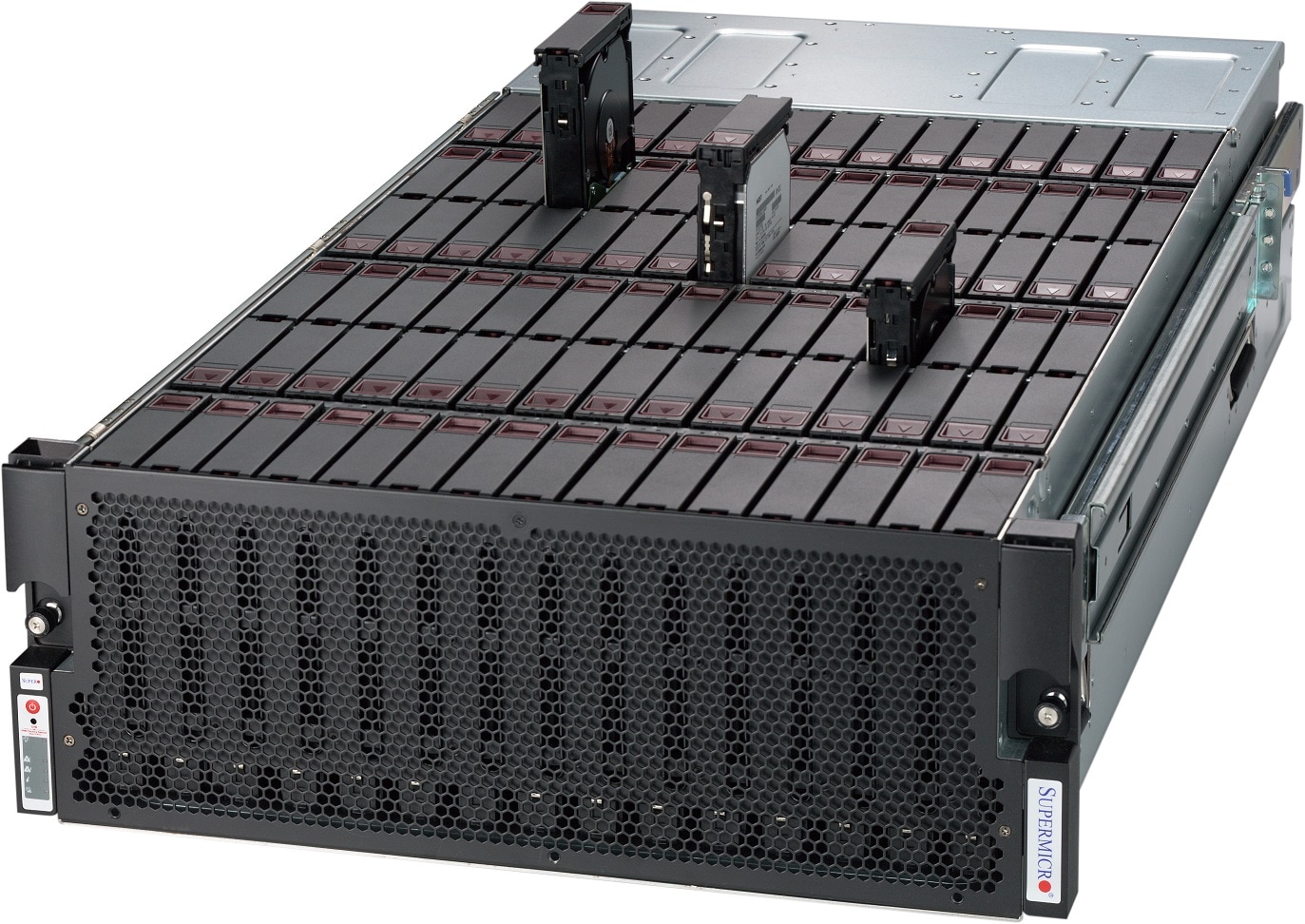
As storage technology has moved on, the filesystems which sit on top of them ideally need to be able to access the full capacity of those ever increasing disks. Many relatively new, or at least in-use, filesystems have serious limitations. Akin to “640K ought to be enough for anybody”, the likes of the FAT32 filesystem supports files which are at most 4GB on a chunk of disk (a partition) which can be at most 16TB. Bear in mind that arrays of disks can provide a working capacity of many times that of a single disk. You can buy the likes of a supermicro sc946ed shelf which will add 90 disks to your server. In an ideal world, as you buy bigger disks you should be able to pile them into your computer and tell your existing filesystem to make use of them, your filesystem should grow and you won’t have to remember a different drive letter or path depending on the hardware you’re using.
ZFS is a 128-bit file system, which means a single installation maxes out at 256 quadrillion zettabytes. All metadata is allocated dynamically so there isn’t the need to pre-allocate inodes and directories can have up to 2^48 (256 trillion) entries. ZFS provides the concept of “vdevs” (virtual devices) which can be a single disk or redundant/striped collections of multiple disks. These can be dynamically added to a pool of vdevs of the same type and your storage will grow onto the fresh hardware.
A further consideration is that both disks of the “spinning rust” variety and SSDs are subject to silent data corruption, i.e. “bit rot”. This can be caused by a number of factors even including cosmic rays, but the consequence is read errors when it comes time to retrieve your data. Manufacturers are aware of this and buried in the small print for your hard disk will be values for “unrecoverable read errors” i.e. data loss. ZFS works around this by providing several mechanisms:
- Checksums for each block of data written.
- Checksums for each pointer to data.
- Scrub – Automatically validates checksums when the system is idle.
- Multiple copies – Even if you have a single disk, it’s possible to provide redundancy by setting a copies=n variable during filesystem creation.
- Self-healing – When a bad data block is detected, ZFS fetches the correct data from a redundant copy and replaces it with the correct data.
An additional bonus to ZFS is its ability to de-duplicate data. Should you be working with a number of very similar files, on a normal filesystem, each file will take up space proportional to the amount of data that’s contained. As ZFS keeps checksums of each block of data, it’s able to determine if two blocks contain identical data. ZFS therefore provides the ability to have multiple pointers to the same file and only store the differences between them.
ZFS also provides the ability to take a point in time snapshot of the entire filesystem and roll it back to a previous time. If you’re a software developer, got a package that has 101 dependencies and you need to upgrade it? Afraid to upgrade it in case it breaks things horribly? Working on code and you want to roll back to a previous version? ZFS snapshots can be run with cron or manually and provide a version of the filesystem which can be used to extract previous versions of overwritten or deleted files or used to roll everything back to a point in time when it worked.

Similar to deduplication, a snapshot won’t take up any disk extra space until the data starts to change.
The other filesystem worth mentioning is tmpfs. Tmpfs takes part of the system memory and turns it into a usable filesystem. This is incredibly useful for systems which create huge numbers of temporary files and attempt to re-read them. Tmpfs is also just about as fast as a filesystem can be. Compared to a single SSD or a RAID array of six disks, tmpfs blows them out of the water speed wise.

Creating a tmpfs filesystem is simple:
First create your mountpoint for the disk:
mkdir /mnt/ramdisk
Then mount it. The options are saying make it 1GB in size, it’s of type tmpfs and to mount it at the previously created mount point:
mount –t tmpfs -o size=1024m tmpfs /mnt/ramdisk
At this point, you can use it like any other filesystem:
df -h
Filesystem Size Used Avail Use% Mounted on
/dev/sda1  218G 128G   80G  62% /
/dev/sdb1  6.3T 2.4T  3.6T  40% /spinnyrust
tank       946G 3.5G  942G   1% /tank
tmpfs      1.0G 391M  634M  39% /mnt/ramdisk
How to parse OAS data
We have recently released the Observed Antibody Space database – collection of cleaned and annotated antibody sequence (Ig-seq or AIRR-seq) data from 53 studies. We have formatted the data in the format that should facilitate data mining and since release we had several queries on how to parse the data out. Therefore here we give a small example of how to parse the data and make sense of it.
You should download the bulk data file from OAS, available here.
The datasets are separated into ‘data units‘ – collections of sequences that can be uniquely assigned to a range of metadata parameters such as study, organism etc. Our task therefore is to iterate through all those files and read sequences from each of these. Firstly we will attempt to iterate through the files and I will assume that you uncompressed the bulk data file into ../data/json folder. We will write a helper function that will simply list all files with its full paths in a directory and call it list_file_paths
import os

#Fetch all files in directory and subdirectories.
def list_file_paths(directory):
   for dirpath,_,filenames in os.walk(directory):
       for f in filenames:
           yield os.path.abspath(os.path.join(dirpath, f))

if __name__ == '__main__':
    #Replace this with the location of where you uncompressed the bulk data file.
    directory = '../data/json'

    for f in list_file_paths(directory):
        print f
The code above will list all the files in ../data/json which incidentally are all the ‘data units’. Now our task is to parse out the output from each of the data units. They are gzipped files with data element on each line. Therefore we will use gzip library to stream the contents of a gzipped file rather than uncompressing each one of them separately. This is achieved by function parse_single_file
import os,gzip

#Fetch all files in directory and subdirectories.
def list_file_paths(directory):
   for dirpath,_,filenames in os.walk(directory):
       for f in filenames:
           yield os.path.abspath(os.path.join(dirpath, f))

#Parse out the contents of a single file.
def parse_single_file(src):
    #The first line are the meta entries.
    meta_line = True
    for line in gzip.open(src,'rb'):
        print line


if __name__ == '__main__':
    #Replace this with the location of where you uncompressed the bulk data file.
    directory = '../data/json'

    for f in list_file_paths(directory):
        parse_single_file(f)
The code above will simply go through all the data unit files, stream the gzipped lines and print each one of them separately. Each line however is formatted as json – meaning it can be parsed using pythons json library and act as a pythonic dictionary. below we have parsed out the basic elements in the final incarnation of the code:
import os,gzip,json,pprint

#Fetch all files in directory and subdirectories.
def list_file_paths(directory):
   for dirpath,_,filenames in os.walk(directory):
       for f in filenames:
           yield os.path.abspath(os.path.join(dirpath, f))

#Parse out the contents of a single file.
def parse_single_file(src):
    #The first line are the meta entries.
    meta_line = True
    for line in gzip.open(src,'rb'):
        if meta_line == True:
                metadata = json.loads(line)
                meta_line=False
                print "Metadata:"
                pprint.pprint(metadata)
                continue
        #Parse actual sequence data.
        basic_data = json.loads(line)
        print "Basic data:"
        pprint.pprint(basic_data)

        #IMGT-Numbered sequence.
        print "IMGT-numbered sequence"
        d = json.loads(basic_data['data'])
        pprint.pprint(d)
        print "==========="

if __name__ == '__main__':
    #Replace this with the location of where you uncompressed the bulk data file.
    directory = '../data/json'

    for f in list_file_paths(directory):
        parse_single_file(f)
The first line of each data unit are meta entries. These look as follows:
{u'Age': u'22-70',
 u'Author': u'Halliley et al., (2015)',
 u'BSource': u'Bone-Marrow',
 u'BType': u'Plasma-B-Cells',
 u'Chain': u'Heavy',
 u'Disease': u'None',
 u'Isotype': u'IGHM',
 u'Link': u'https://doi.org/10.1016/j.immuni.2015.06.016',
 u'Longitudinal': u'no',
 u'Size': 934,
 u'Species': u'human',
 u'Subject': u'no',
 u'Vaccine': u'Tetanus/Flu'}
The attributes should be self-explanatory and the existence of this data on top of each file is supposed to streamline searching through data-units if you wish to parse sequences given a particular configuration of meta-data entries (e.g. organism).
Next, the code parses out data on each sequence that is associated with its genes, full sequence, CDR3 and numbered sequence. Therefore the output for this will look something like this:
{u'cdr3': u'ARHQGVYWVTTAGLSH',
 u'data': u'{"fwh1": {"11": "G", "24": "T", "13": "V", "12": "L", "15": "P", "14": "K", "17": "E", "16": "S", "19": "L", "18": "T", "22": "T", "26": "S", "25": "V", "21": "L", "20": "S", "23": "C"}, "fwh3": {"68": "N", "88": "S", "89": "L", "66": "Y", "67": "Y", "82": "T", "83": "S", "80": "V", "81": "D", "86": "Q", "87": "F", "84": "K", "85": "N", "92": "S", "79": "S", "69": "P", "104": "C", "78": "I", "77": "T", "76": "V", "75": "R", "74": "S", "72": "K", "71": "L", "70": "S", "102": "Y", "90": "K", "100": "A", "101": "V", "95": "T", "94": "V", "97": "A", "96": "A", "91": "L", "99": "T", "98": "D", "93": "S", "103": "Y"}, "fwh2": {"52": "W", "39": "W", "48": "Q", "49": "G", "46": "P", "47": "G", "44": "Q", "45": "P", "51": "E", "43": "R", "40": "G", "42": "I", "55": "S", "53": "I", "54": "G", "41": "W", "50": "L"}, "fwh4": {"120": "Q", "121": "G", "122": "T", "123": "L", "124": "V", "125": "P", "126": "V", "127": "S", "128": "S", "119": "G", "118": "W"}, "cdrh1": {"27": "G", "37": "Y", "31": "S", "30": "I", "28": "G", "29": "S", "35": "S", "34": "S", "38": "Y", "36": "S"}, "cdrh2": {"59": "S", "58": "Y", "57": "S", "56": "I", "63": "G", "64": "T", "65": "T"}, "cdrh3": {"111A": "W", "109": "G", "108": "Q", "115": "L", "114": "G", "117": "H", "116": "S", "111": "Y", "110": "V", "113": "A", "112": "T", "112A": "T", "112B": "V", "106": "R", "107": "H", "105": "A"}}',
 u'j': u'IGHJ1*01',
 u'name': 12,
 u'redundancy': 1,
 u'seq': u'GLVKPSETLSLTCTVSGGSISSSSYYWGWIRQPPGQGLEWIGSISYSGTTYYNPSLKSRVTISVDTSKNQFSLKLSSVTAADTAVYYCARHQGVYWVTTAGLSHWGQGTLVPVSS',
 u'v': u'IGHV4-39*07'}
Above, redundancy refers to how many times we see a given sequence (seq) in a particular study. We also store the IMGT-numbered data (the data attribute) which needs a second round of json parsing and its output is a dictionary of IMGT-number – amino acid associations grouped by the regions of an antibody (cdrs and framework regions):
{u'cdrh1': {u'27': u'G',
            u'28': u'G',
            u'29': u'S',
            u'30': u'I',
            u'31': u'S',
            u'34': u'S',
            u'35': u'S',
            u'36': u'S',
            u'37': u'Y',
            u'38': u'Y'},
 u'cdrh2': {u'56': u'I',
            u'57': u'S',
            u'58': u'Y',
            u'59': u'S',
            u'63': u'G',
            u'64': u'T',
            u'65': u'T'},
 u'cdrh3': {u'105': u'A',
            u'106': u'R',
            u'107': u'H',
            u'108': u'Q',
            u'109': u'G',
            u'110': u'V',
            u'111': u'Y',
            u'111A': u'W',
            u'112': u'T',
            u'112A': u'T',
            u'112B': u'V',
            u'113': u'A',
            u'114': u'G',
            u'115': u'L',
            u'116': u'S',
            u'117': u'H'},
 u'fwh1': {u'11': u'G',
           u'12': u'L',
           u'13': u'V',
           u'14': u'K',
           u'15': u'P',
           u'16': u'S',
           u'17': u'E',
           u'18': u'T',
           u'19': u'L',
           u'20': u'S',
           u'21': u'L',
           u'22': u'T',
           u'23': u'C',
           u'24': u'T',
           u'25': u'V',
           u'26': u'S'},
 u'fwh2': {u'39': u'W',
           u'40': u'G',
           u'41': u'W',
           u'42': u'I',
           u'43': u'R',
           u'44': u'Q',
           u'45': u'P',
           u'46': u'P',
           u'47': u'G',
           u'48': u'Q',
           u'49': u'G',
           u'50': u'L',
           u'51': u'E',
           u'52': u'W',
           u'53': u'I',
           u'54': u'G',
           u'55': u'S'},
 u'fwh3': {u'100': u'A',
           u'101': u'V',
           u'102': u'Y',
           u'103': u'Y',
           u'104': u'C',
           u'66': u'Y',
           u'67': u'Y',
           u'68': u'N',
           u'69': u'P',
           u'70': u'S',
           u'71': u'L',
           u'72': u'K',
           u'74': u'S',
           u'75': u'R',
           u'76': u'V',
           u'77': u'T',
           u'78': u'I',
           u'79': u'S',
           u'80': u'V',
           u'81': u'D',
           u'82': u'T',
           u'83': u'S',
           u'84': u'K',
           u'85': u'N',
           u'86': u'Q',
           u'87': u'F',
           u'88': u'S',
           u'89': u'L',
           u'90': u'K',
           u'91': u'L',
           u'92': u'S',
           u'93': u'S',
           u'94': u'V',
           u'95': u'T',
           u'96': u'A',
           u'97': u'A',
           u'98': u'D',
           u'99': u'T'},
 u'fwh4': {u'118': u'W',
           u'119': u'G',
           u'120': u'Q',
           u'121': u'G',
           u'122': u'T',
           u'123': u'L',
           u'124': u'V',
           u'125': u'P',
           u'126': u'V',
           u'127': u'S',
           u'128': u'S'}}
We hope this quick intro to our data format will allow you to do great science with this data.
Working with Jupyter notebook on a remote server
To celebrate the recent beta release of Jupyter Lab (try it out of you haven’t already), today we’re going to look at how to run a Jupyter session (Notebook or Lab) on a remote server.
Suppose you have lots of data which lives on a remote server and you want to play with it in a Jupyter notebook. You can’t copy the data to your local machine (well, you can, but you’re sensible so you won’t), but you can run your Jupyter session on the remote server. There’s just one problem – since Jupyter notebook is browser-based and works by connecting to the Jupyter session running locally, you can’t just run Jupyter remotely and forward X11 like you would a traditional graphical IDE. Fortunately, the solution is simple: we run Jupyter remotely, create an ssh tunnel connecting a local port to the one used by the Jupyter session, and connect directly to the Jupyter session using our local browser. The best part about this is that you can set up the Jupyter session once then connect to it from any browser on any machine once an ssh tunnel is created, without worrying about X11 forwarding.
Here’s how to do it.
1. First, connect to the remote server if you haven’t already
ssh fergus@funkyserver
1.5. Jupyter takes browser security very seriously, so in order to access a remote session from a local browser we need to set up a password associated with the remote Jupyter session. This is stored in jupyter_notebook_config.py which by default lives in ~/.jupyter. You can edit this manually, but the easiest option is to set the password by running Jupyter with the password argument:
jupyter notebook password
>>> Enter password:
This password will be used to access any Jupyter session running from this installation, so pick something sensible. You can set a new password at any time on the remote server in exactly the same way.
2: Launch a Jupyter session on the remote server. You can specify the access port using the --port option. This might be useful on a shared server where others might be doing the same thing. You’ll also want to run this without launching a browser on the remote server since this is of no use to you.
jupyter lab --port=9000 --no-browser &
Here I’m using Jupyter Lab, but this works in exactly the same way for Jupyter Notebook.
3: Now for the fun part. Jupyter is running on our remote server, but what we really want is to work in our favourite browser on our local machine. To do this we just need to create an ssh tunnel between a port on our machine and the port our Jupyter session is using on the remote server. On our local machine:
ssh -N -f -L 8888:localhost:9000 fergus@funkyserver
For those not familiar with ssh tunneling, we’ve just created a secure, encrypted connection between port 8888 on our local machine and port 9000 on our remote server.
- -N tells ssh we won’t be running any remote processes using the connection. This is useful for situations like this where all we want to do is port forwarding.
- -f runs ssh in the background, so we don’t need to keep a terminal session running just for the tunnel.
- -L specifies that we’ll be forwarding a local port to a remote address and port. In this case, we’re forwarding port 8888 on our machine to port 9000 on the remote server. The name ‘localhost’ just means ‘this computer’. If you’re a Java programmer who lives for verbosity, you could equivalently pass
-L localhost:8888:localhost:9000.
4: If you’ve done everything correctly, you should now be able to access your Jupyter session via port 8888 on your machine. Fire up your favourite browser and type localhost:8888 into the address bar. This should bring up a Jupyter session and prompt you for a password. Enter the password you specified for Jupyter on the remote server.
Congratulations! You now have a Jupyter session running remotely which you can connect to anytime, anywhere, from any machine.
Disclaimer: I haven’t tried this on Windows, nor do I intend to. I value my sanity.
Dealing with indexes when processing co-evolution signals (or how to navigate through “sequence hell”)
Co-evolution techniques provide a powerful way to extract structural information from the wealth of protein sequence data that we now have available. These techniques are predicated upon the notion that residues that share spatial proximity in a protein structure will mutate in a correlated fashion (co-evolve). This co-evolution signal can be inferred from a multiple sequence alignment, which tells us a bit about the evolutionary history of a particular protein family. If you want to have a better gauge at the power of co-evolution, you can refer to some of our previous posts (post1, post2).
This is more of a practical post, where I hope to illustrate an indexing problem (and how to circumvent it) that one commonly encounters when dealing with co-evolution signals.
Most of the co-evolution tools available Today output pairs of residues (i,j) that were predicted to be co-evolving from a multiple sequence alignment. One of the main applications of these techniques is to predict protein contacts, that is pairs of residues that are within a predetermined distance (quite often 8Å). Say you want to compare the precision of different co-evolution methods for a particular test set. Your test set would consist of a number of proteins for which the structure is known and for which sufficient sequence information is available for the contact prediction to be carried out. Great!
So you start with your target sequences, generate a number of contact predictions of the form (i,j) for each sequence and, for each pair, you check if the ith and jth residues are in contact (say, less than 8Å apart) on the corresponding known protein structure. If you actually carry out this test, you will obtain appalling precision for a large number of test cases. This is due to an index disparity that a friend of mine quite aptly described as “sequence hell”.
This indexing disparity occurs because there is a mismatch between the protein sequence that was used to produce the contact predictions and the sequence of residues that are represented in a protein structure. Ask a crystallographer friend if you have one, and you will find that in the process of resolving a protein’s structure experimentally, there are many reasons why residues would be missing in the final structure. More so, there are even cases where residues had to be added to enable protein expression and/or crystallisation. This implies that the protein sequence (represented by a fasta file) frequently has more (and sometimes fewer) residues than the proteins structure (represented by a PDB file). This means that if the ith and jth residues in your sequence were predicted to be in contact, that does not mean that they correspond to the ith and jth residues in order of appearance in your protein structure. So what do we do now?
A true believer in the purity and innocence of the world would assume that the SEQRES entries in your PDB file, for instance, would come to the rescue. The SEQRES describes the sequence of residues exactly as they appear on the atom coordinates of a particular PDB file. This would be a great way of mitigating the effects of added or altered residues, and would potentially mitigate the effects of residues that were not present in the construct. In other words, the sequences described by SEQRES would be a good candidate to validate whether your predicted contacts are present in the structure. They do, however, contain one limitation. SEQRES also describe any residues whose coordinates were missing in the PDB. This means that if you process the PDB sequentially and that some residues could not be resolved, the ith residue to appear on the PDB could be different to the ith residue in the SEQRES.
An even more innocent person, shielded from all the ugliness of the the universe, would simply hope that the indexing on the PDB is correct, i.e. that one can use the residue indexes presented on the “6th column” of the ATOM entries and that these would match perfectly to the (i,j) pair you obtained using your protein sequence. While, in theory, I believe this should be the case, in my experience this indexing is often incorrect and more frequently than not, will lead to errors when validating protein contacts.
My solution to the indexing problem is to parse the PDB sequentially and extract the sequence of all the residues for which coordinates are actually present. To my knowledge, this is the only true and tested way of obtaining this information. If you do that, you will be armed with a sequence and indexing that correctly represent the indexing of your PDB. From now on, I will refer to these as the PDB-sequence and PDB-sequence indexing.
All that is left is to find a correspondence (a mapping) between the sequence you used for the contact prediction and the PDB-sequence. I do that by performing a standard (global) sequence alignment using the Needleman–Wunsch algorithm. Once in possession of such an alignment, the indexes (i,j) of your original sequence can be matched to adjusted indexes (i',j') on your PDB-sequence indexing. In short, you extracted a sequential list of residues as they appeared on the PDB, aligned these to the original protein sequence, and created a new set of residue pairings of the form (i',j') which are representative of the indexing in PDB-sequence space. That means that the i’th residue to appear on the PDB was predicted to be in contact with the j’th residue to appear.
The problem becomes a little more interesting when you hope to validate the contact predictions for other proteins with known structure in the same protein family. A more robust approach is to use the sequence alignment that is created as part of the co-evolution prediction as your basis. You then identify the sequence that best represents the PDB-sequence of your homologous protein by performing N global sequence alignments (where N is the number of sequences in your MSA), one per entry of the MSA. The highest scoring alignment can then be used to map the indexing. This approach is robust enough that if your homologous PDB-sequence of interest was not present in the original MSA for whatever reason, you should still get a sensible mapping at the end (all limitations of sequence alignment considered).
One final consideration should be brought to the reader’s attention. What happens if, using the sequence as a starting point, one obtains one or more (i,j) pairs where either i or j is not resolved/present in the protein structure? For validation purposes, often these pairs are disregards. Yet, what does this co-evolutionary signal tell us about the missing residues in the structure? Are they disordered/flexible? Could the co-evolution help us identify low occupancy conformations?
I’ll leave the reader with these questions to digest. I hope this post proves helpful to those braving the seas of “sequence hell” in the near future.
Interactive Illustration of Collaboration Networks with D3
D3 is a JavaScript Library that allows the creation of interactive data visualisations. D3 stands for Data-Driven Documents and its advantage is that it is using internet standards as HTML, CSS, and SVG as the foundation. This gives maximal compatibility across all moderns browsers. It is widely used by journalists, data scientists, and starts to be used by academic scientists, too.
Here I want to present a simple way of creating interactive illustrations of collaboration networks, e.g., for your own website. Before going into details, have a look at the example below, it presents some of Rosalind Franklin’s papers and her co-authors.
[d3-source canvas=”wpd3-3903-2″]
The network illustration is a so-called bipartite network because it consists of two types of nodes, blue nodes represent scientists and orange nodes represent publications. These nodes are connected if a scientist is an author on a publication. This way of presenting is a so-called force layout, which simulates repelling Coulomb forces between all nodes and spring-like attractive forces act on nodes that are connected via links. You can drag the nodes around and explore the behaviour of the network.
You will have noticed that you can also see the name of the publications and co-authors when you hover over the nodes. For some of them, a representative figure or photograph is shown, too. You can also double-click the nodes and will be directed to the webpage of the publication or author.
For larger collaboration networks the visualisation is still possible but might get a bit messy. Thus, not showing any figures is advised. Furthermore, the name of the nodes should be shown either below the illustration or as a tooltip (the later is not possible in WordPress but on normal web pages as here). The illustration below shows all 124 publications written by OPIG, together with the 310 authors. Here, I had to remove the Head of the Group Charlotte Deane, as she is on almost all of these papers and would clutter the illustration, unfortunately. In network science, we call such a node an ego node.
[d3-source canvas=”wpd3-3903-0″]
If you want to play around with this, check out my Github repository. The creation of the network is fairly simple. You only need a Bibtex file and can then execute a Python script that creates a JSON file that is read into the JavaSript. This can then be incorporated in all web pages easily.
PS: To enable D3 in WordPress you need a special plugin. Apparently, it is not up to date with the current stable D3 version 4 but you can load any missing functions manually.
Crystallographic programming: Super short tour of the cctbx
Two of the leading packages in crystallography are Phenix and CCP4. For most practicing crystallographers they will interact via with these to progress a single crystallographic data-set from diffraction images, through integration, merging, phasing, model building and hopefully deposition.

However, if you want to develop crystallographic software, you will likely need to decide on a framework to build upon. Phenix is built on the comprehensive cctbx library, whereas CCP4 programs are typically standlone, although common crystallographic libraries such as clipper and cctbx are utilised.
CCTBX is written mainly in python, with core crystallographic functionality written in C++. My usual starting place for understanding functionality is through the pdb parser tutorial. This introduces the concept of a hierarchy, a iterative way to represent a macromolecule:
from iotbx.pdb import hierarchy
pdb_in = hierarchy.input(file_name="model.pdb")
for chain in pdb_in.hierarchy.only_model().chains() :
  for residue_group in chain.residue_groups() :
    for atom_group in residue_group.atom_groups() :
      for atom in atom_group.atoms() :
        if (atom.element.strip().upper() == "ZN") :
          atom_group.remove_atom(atom)
      if (atom_group.atoms_size() == 0) :
        residue_group.remove_atom_group(atom_group)
    if (residue_group.atom_groups_size() == 0) :
      chain.remove_residue_group(residue_group)
f = open("model_Zn_free.pdb", "w")
f.write(pdb_in.hierarchy.as_pdb_string(
  crystal_symmetry=pdb_in.input.crystal_symmetry()))
f.close()
Although there are many ways to parse a pdb file, the introduction to iotbx.pdb, gives a view of how xray structure data can be associated to the model. The tour of the cctbx can be helpful starting place, especially for understanding how the python and c++ functionality interact through boost and the scitbx.array_family.flex. Unfortunately, documentation on cctbx tends to vary in quality and quantity throughout the modules:
- libtbx – low-level utilities and infrastructure for CCTBX
- boost_adaptbx – wrappers for Boost functionality
- iotbx – file readers and writers
- scitbx – general-purpose scientific programming infrastructure
- cctbx – core crystallographic objects and functions
- mmtbx – macromolecular crystallography
Other components of the library include ways to simulate crystallographic data through simtbx, and tools for processing xfel data.
As the library is open source, github hosted source code allows exploration of previously written routines, which can be very helpful for understanding the inner workings of the library. Note that there are also bulletin boards for users and developers of phenix and cctbx respectively. A few tutorials can also be found.
Hopefully this post will give someone other than me a reminder of where to find resources to get started developing within CCTBX.
Latexing with gvim
Here I’ll share my set-up for writing Latex with gvim instead of a separate Latex editor. If you are text-editor averse, this blog post is not for you. But if, like me, you love vim and hate useless GUIs, this might be helpful.
We’re lucky to have nice big screens in the Stats Department, but I tend to prefer writing on my MacBook (I find it’s easier to transport to e.g. a cafe, my home, etc). Until now, I’ve been happily using TexMaker for writing, but during a recent period of intense Latexing I started to find the useable screen space oppressively small. The unnecessary GUI had to go.

No offence TexMaker but I don’t like you
One of our good friends in Statistical Genetics recommended some things to help me with the transition to just using good old (g)vim, which I will now recommend to you.
The key thing is the LaTex-Box plug-in for vim, which gives you the compilation commands, as well as the essentials such as smart indentation, highlight matching, command completion, etc. I used pathogen to install it (see the GitHub for instructions).
Of course, you can then customise your .vimrc file to add more helpful things. This can be the simple preferences, such as using a light background when using gvim:
if has(“gui_running”)

        set background=light

endif
You can also do more complicated magic like tabbing through available commands, and the ability to minimise sections, etc. Sidenote: to make working with paragraphs easier, I recommend setting the up/down arrows to move the cursor to the next line in the GUI rather than the next actual line. I prefer overriding this behaviour only in gvim, while leaving the normal behaviour in vim (for actual coding). But each to their own.
To get started, open a .tex file, then compile and view the document with the command Latexmk.

Command suggestions are an example of a magical feature added in .vimrc
The configurations for this command are set in the file .latexmkrc. Mine looks like this:
$recorder = 1;
$pdf_mode = 1;
$bibtex_use = 2;
$pdflatex = "pdflatex --shell-escape %O %S";
$pdf_previewer = "start open -a skim %O %S";
My pdf viewer of choice on Mac is Skim, which autoupdates. I view the source and preview at the same time using split view. Please admire the beauty below:

Wow what a beautiful screen
My favourite part is that whenever you save (w), it recompiles and updates the preview. As someone who accidentally types :w everywhere that isn’t vim, it’s nice that this is now productive. It also recompiles automatically if the .bib file is updated. Note that if you have errors at compilation (I’m sure you don’t), you can view them with the command LatexErrors.
Now you too can be a (nearly) GUI-free lightweight Latexer. Enjoy!