Category Archives: Group Meetings

What we discuss during cake at our Tuesday afternoon group meetings

Biophysical Society 61st Annual Meeting – New Orleans, February 2017

As the sole representative of OPIG attending Biophys 2017 in New Orleans, I had to bear the heavy burden of a long and lonely flight and the fear of missing out on a week of the very grey Oxford winter. Having successfully crossed the border into the US, which was thankfully easier for me than it was for some of our scientific colleagues from around the world, I found my first time attending the conference to be full of very interesting and relevant science. While also covering a wide variety of experimental techniques and non-protein topics, the conference is so large and broad that there was more than enough to keep me busy over the five days, featuring folding, structure prediction, docking, networks, and molecular dynamics.

There were several excellent talks on the subject of folding pathways, misfolding and aggregation. A common theme was the importance of the kinetic stability of the native state, and the mechanisms by which it may be prevented from reaching a non-native global thermodynamic minimum. This is particularly important for serpins, large protease inhibitors which inactivate proteases by a suicide mechanism. The native and active state can be transformed into a lower energy conformation over long timescales. However, this also occurs by cleavage near the C-terminal end, which allows insertion of the C-terminal tail into a beta sheet, holding the cleaving protease inactive and therefore the stored energy is very important for function. Anne Gershenson described recent simulations and experiments to elucidate the order in which substructures of the complete fold assemble. There are many cooperative substructures in this case, and N-terminal helices form at an early stage. The overall topology appears to be consistent with a cotranslational folding mechanism inside the ER, but requires significant rearrangements after translation for adoption of the full native fold.

Cotranslational folding was also discussed by several others including the following: Patricia Clark is now using the YKB system of alternately folding fluorescent protein to find new translation stalling sequences; Anais Cassaignau described NMR experiments to show the interactions taking place between nascent chains and the ribosome at different stalled positions during translation; and Daniel Nissley presented a model to predict a shift in folding mechanism from post-translational to cotranslational due to specific designed synonymous codon changes, which agreed very well with experimental data.

To look more deeply into the evolution of folding mechanisms and protein stability, Susan Marqusee presented a study of the kinetics of folding of RNases, comparing the properties of inferred ancestral sequences to a present day thermophile and mesophilic E. coli. A number of reconstructed sequences were expressed, and it was found that moving along either evolutionary branch from the ancestor to modern day, folding and unfolding rates had both decreased, but the same three-state folding pathway via an intermediate is conserved for all ancestors. However, the energy transition between the intermediate and the unfolded state has evolved in opposite directions even while the kinetic stability remains similar. This has led to the greater thermodynamic stability seen in the modern day thermophile compared to the mesophile at higher temperatures and concentrations of denaturant.

Panel C shows that kinetic stability (low unfolding rate) seems to be selected for in both environments. Panel D shows that the thermodynamic stability of the intermediate (compared to the unfolded state) accounts for the differences in thermodynamic stability of the native state, when compared to the common ancestor (0,0). Link to paper

There were plenty of talks discussing the problems and mechanisms of protein aggregation, with two focussing on light chain amyloidosis. Marina Ramirez-Alvarado was investigating how fibrils begin to grow and showed using microscopy that both soluble light chains and fibrils (more slowly) are internalised by heart muscle cells. They can then be exposed at the cell surface and become a seed to recruit other soluble light chains to form fibrils. Shannon Esswein presented work on the enhancement of VL-VL dimerisation to prevent amyloid formation. The variable domain of the light chain (VL) can pair with itself in a similar orientation to its pairing with VH domains in normal antibodies, or in a non-canonical orientation. Adding disulphide bonds to stabilise these dimers prevented fibril formation, therefore they carried out a small scale screen of 27 aromatic and hydrophobic ligands to find those which would favour dimer formation by binding at the interface. Sulfasalazine was detected in this screen and was also shown to significantly reduce fibril formation and could therefore be used as a template for future drug design.

A ligand stabilises the dimer therefore fewer light chains are present as monomers, slowing the rate of the only route by which fibrils can be formed. Link to paper

Among the posters, Alan Perez-Rathke presented loop modelling by DiSGro in beta barrel membrane proteins which showed that the population of structures generated and scored favourably after relaxation at a pH 7 led to an open pore more often than at pH 5, consistent with experimental observations. There were two posters on the topic of prediction of membrane protein expression in bacteria and yeast presented by students of Bill Clemons, who also gave a great talk. Shyam Saladi has carefully curated datasets of successes and failures in expression in E. coli and trained a linear SVM on features such as RNA secondary structure and transmembrane segment hydrophobicity to predict the outcome for unknown proteins. This simple approach (preprint available here) achieved area under ROC curve of around 0.6 on a separate test set, and using more complex machine learning techniques is likely to improve this. Samuel Schulte is adapting the same method for prediction of expression in yeast.

Overall, it was a great conference and it was nice to hear about plenty of experimental work alongside the more familiar computational work. I would also highly recommend New Orleans as an excellent place to find great food, jazz and sunshine!

Using Antibody Next Generation Sequencing data to aid antibody engineering

       I consider myself a wet lab scientist and I had not done any dynamic programming language like Python before starting my DPhil. My main interests lie in development of improved antibody humanization campaigns, rational antibody phage display library constructions and antibody evolution. Having completed industrial placement at MedImmune, I saw the biotechnology industry from the inside and realized that scientists who could bridge computer science and wet lab fields are in high demand.

      The title of my DPhil is very broad, and research itself is data rather than hypothesis driven. Our research group collaborates with UCB Pharma, which has sequenced whole antibody repertoires across a number of species. Datasets might contain more than 10 million sequences of heavy and light variable chains. But even these datasets do not cover more than 1% of the theoretical repertoire, hence looking at entropies of sequences rather than mere sequences could provide insights into differences between intra- and inter- species datasets.

        NGS of antibody repertoires provides snapshots of repertoire diversity, entropy as well as sequences. Reddy, S.T. et al 2010 showed that this information could be successfully used to pull target specific variable chains. But most of research groups believe that main application of NGS is immunodiagnostics (Grieff et al., 2015).

       My project involves applying software developed by our research group namely, Anarci (Dunbar J and Deane CM., 2016) and ABodyBuilder (Leem J. et al 2016). Combination of both softwares allows analysis of NGS datasets at an unprecedented rate (1 million sequences per 7 hours). A number of manipulations can be performed on datasets to standardize them and make data reproducible, which is a big issue in science. It is possible to re-assign germlines, numbering schemes and complementary determining region (CDR) definitions of a 10 million dataset in less than a day. For instance, UCB provided data required our variable chains to be re-numbered according to IMGT numbering and CDR definition (Lefranc M., 2011). The reason for the IMGT numbering scheme selection is that it supports symmetrical amino acid numbering of CDRs, which allows for improved assignment of positions to amino acids that are located in the same structural space between different length CDRs (Figure 1).

                Figure 1. IMGT numbering and CDR definition of CDR3. Symmetrical assignment of positions to amino acids in HCDR3 allows for better localization of V,D,J genes: V gene encodes for the amino terminus, J gene encodes the carboxyl terminus of CDR3, and D gene the mid portion.

       To sum up, analysis of CDR lengths, CDR and framework amino acid compositions, finding novel patterns in antibody repertoires will open up new rational steps of antibody humanization and affinity maturation. The key step will be to determine amino acid scaffolds that define humanness of antibody or in other words, scaffolds that are not immunogenic in humans.

References:

  1. Dunbar J., and Deane CM., ANARCI: Antigen receptor numbering and receptor classification. Bioinformatics (2016)
  2. Grieff V., A bioinformatic framework for immune repertoire diversity profiling enables detection of immunological status. Genome Medicine (2015)
  3. Leem J., et al. ABodyBuilder: automated antibody structure prediction with data-driven accuracy estimation. mAbs. (2016)
  4. Lefranc M., IMGT, the International ImMunoGeneTics Information System. Cold Spring Harb Protoc. (2011)
  5. Reddy ST., et al. Monoclonal antibodies isolated without screening by analyzing the variable-gene repertoire of plasma cells. Nat Biotech. (2010)

Multiomics data analysis

Cells are the basic functional and structural units of living organisms. They are the location of many different biological processes, which can be probed by various biological techniques. Until recently such data sets have been analysed separately. The aim is to better understand the underlying biological processes and how they influence each other. Therefore techniques that integrate the data from different sources might be applicable [1].

In the image below you see the four main entities that are active throughout the cell: Genome, RNA, proteins, and metabolites. All of them are in constant interaction, for example, some proteins are transcription factors and influence the transcription of DNA into RNA. Metabolites that are present in the cell also influence the activity of proteins as ligands but at the same time are altered through enzymatic activity. This ambiguity of interactions makes it clear that probing the system at a single level gives only limited insight into the structure and function of the cellular processes.


multiomics_schematic

The different levels of biological information (genome, proteome, …) work mutually and influence each other through processes as transcription regulation through transcription factors. All levels are influenced by external factors, as drug treatment or nutrient availability. Multiomics is the measurement of multiple of those populations and their integrated analysis.

In the last years, different ways to integrate such data have been developed. Broadly speaking there are three levels of data integration: conceptual integration, statistical integration, and model-based integration [2]. Conceptual integration means that the data sets are analysed separately and the conclusions are compared and integrated. This method can easily use already existing analysis pipelines but the way in which conclusions are compared and integrated is non-trivial. Statistical Integration combines data sets and analyses them jointly, reaching conclusions that match all data and potentially finding signals that are not observable with the conceptual approach. Model-based integration indicates the joint analysis of the data in a combination of training of a model, which itself might incorporate prior beliefs of a system.

[1] Gehlenborg, Nils, Seán I. O’donoghue, Nitin S. Baliga, Alexander Goesmann, Matthew A. Hibbs, Hiroaki Kitano, Oliver Kohlbacher et al. “Visualization of omics data for systems biology.” Nature methods 7 (2010): S56-S68.

[2] Cavill, Rachel, Danyel Jennen, Jos Kleinjans, and Jacob Jan Briedé. “Transcriptomic and metabolomic data integration.” Briefings in bioinformatics 17, no. 5 (2016): 891-901.

Prions

The most recent paper presented to the OPIG journal club from PLOS Pathogens, The Structural Architecture of an Infectious Mammalian Prion Using Electron Cryomicroscopy. But prior to that, I presented a bit of a background to prions in general.

In the 1960s, work was being undertaken by Tikvah Alper and John Stanley Griffith on the nature of a transmissible infection which caused scrapie in sheep. They were interested in how studies of the infection showed it was somehow resistant to ionizing radiation. Infectious elements such as bacteria or viruses were normally destroyed by radiation with the amount of radiation required having a relationship with the size of the infectious particle. However, the infection caused by the scrapie agent appeared to be too small to be caused by even a virus.

In 1982, Stanley Prusiner had successfully purified the infectious agent, discovering that it consisted of a protein. “Because the novel properties of the scrapie agent distinguish it from viruses, plasmids, and viroids, a new term “prion” was proposed to denote a small proteinaceous infectious particle which is resistant to inactivation by most procedures that modify nucleic acids.”
Prusiner’s discovery led to him being awarded the Nobel Prize in 1997.

Whilst there are many different forms of infection, such as parasites, bacteria, fungi and viruses, all of these have a genome. Prions on the other hand are just proteins. Coming in two forms, the naturally occurring cellular (PrPC) and the infectious form PrPSC (Sc referring to scrapie), through an as yet unknown mechanism, PrPSC prions are able to reproduce by forcing beneign PrPC forms into the wrong conformation.  It’s believed that through this conformational change, the following diseases are caused.

  • Bovine Spongiform encephalopathy (mad cow disease)
  • Scrapie in:
    • Sheep
    • Goats
  • Chronic wasting disease in:
    • Deer
    • Elk
    • Moose
    • Reindeer
  • Ostrich spongiform encephalopathy
  • Transmissible mink encephalopathy
  • Feline spongiform  encephalopathy
  • Exotic ungulate encephalopathy
    • Nyala
    • Oryx
    • Greater Kudu
  • Creutzfeldt-Jakob disease in humans


Whilst it’s commonly accepted that prions are the cause of the above diseases there’s still debate whether the fibrils which are formed when prions misfold are the cause of the disease or caused by it. Due to the nature of prions, attempting to cure these diseases proves extremely difficult. PrPSC is extremely stable and resistant to denaturation by most chemical and physical agents. “Prions have been shown to retain infectivity even following incineration or after being subjected to high autoclave temperatures“. It is thought that chronic wasting disease is normally transmitted through the saliva and faeces of infected animals, however it has been proposed that grass plants bind, retain, uptake, and transport infectious prions, persisting in the environment and causing animals consuming the plants to become infected.

It’s not all doom and gloom however, lichens may long have had a way to degrade prion fibrils. Not just a way, but because it’s apparently no big thing to them, have done so twice. Tests on three different lichens species: Lobaria pulmonaria, Cladonia rangiferina and Parmelia sulcata, indicated at least two logs of reduction, including reduction “following exposure to freshly-collected P. sulcata or an aqueous extract of the lichen”. This has the potential to inactivate the infectious particles persisting in the landscape or be a source for agents to degrade prions.

Using RDKit to load ligand SDFs into Pandas DataFrames

If you have downloaded lots of ligand SDF files from the PDB, then a good way of viewing/comparing all their properties would be to load it into a Pandas DataFrame.

RDKit has a very handy function just for this – it’s found under the PandasTool module.

I show an example below within Jupypter-notebook, in which I load in the SDF file, view the table of molecules and perform other RDKit functions to the molecules.

First import the PandasTools module:

from rdkit.Chem import PandasTools

Read in the SDF file:

SDFFile = "./Ligands_noHydrogens_noMissing_59_Instances.sdf"
BRDLigs = PandasTools.LoadSDF(SDFFile)

You can see the whole table by calling the dataframe:

BRDLigs

The ligand properties in the SDF file are stored as columns. You can view what these properties are, and in my case I have loaded 59 ligands each having up to 26 properties:

BRDLigs.info()

It is also very easy to perform other RDKit functions on the dataframe. For instance, I noticed there is no heavy atom column, so I added my own called ‘NumHeavyAtoms’:

BRDLigs['NumHeavyAtoms']=BRDLigs.apply(lambda x: x['ROMol'].GetNumHeavyAtoms(), axis=1)

Here is the column added to the table, alongside columns containing the molecules’ SMILES and RDKit molecule:

BRDLigs[['NumHeavyAtoms','SMILES','ROMol']]

Confidence (scores) in STRING

There are many techniques for inferring protein interactions (be it physical binding or functional associations), and each one has its own quirks: applicability, biases, false positives, false negatives, etc. This means that the protein interaction networks we work with don’t map perfectly to the biological processes they attempt to capture, but are instead noisy observations.

The STRING database tries to quantify this uncertainty by assigning scores to proposed protein interactions based on the nature and quality of the supporting evidence. STRING contains functional protein associations derived from in-house predictions and homology transfers, as well as taken from a number of externally maintained databases. Each of these interactions is assigned a score between zero and one, which is (meant to be) the probability that the interaction really exists given the available evidence.

Throughout my short research project with OPIG last year I worked with STRING data for Borrelia Hermsii, a relatively small network of scored interactions across 815 proteins. I was working with v.10.0., the latest available database release, but also had the chance to compare this to v.9.1 data. I expected that with data from new experiments and improved scoring methodologies available, the more recent network would be more or less a re-scored superset of the older. Even if some low-scored interactions weren’t carried across the update, I didn’t expect these to be any significant proportion of the data. Interestingly enough, this was not the case.

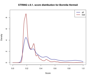
Out of 31 264 scored protein-protein interactions in v.9.1. there were 10 478, i.e. almost exactly a third of the whole dataset, which didn’t make it across the update to v.10.0. The lost interactions don’t seem to have very much in common either — they come from a range of data sources and don’t appear to be located within the same region of the network. The update also includes 21 192 previously unrecorded interactions.

densityComparison

Gaussian kernel density estimates for the score distribution of interactions across the entire 9.1. Borrelia Hermsii dataset (navy) and across the discarded proportion of the dataset (dark red). Proportionally more low-scored interactions have been discarded.

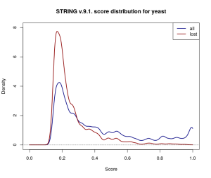
Repeating the comparison with baker’s yeast (Saccharomyces cerevisiae), a much more extensively studied organism, shows this isn’t a one-off case either. The yeast network is much larger (777 589 scored interactions across 6400 proteins in STRING v.9.1.), and the changes introduced by v.10.0. appear to be scaled accordingly — 237 427 yeast interactions were omitted in the update, and 399 836 new ones were added.

discardedYeast

Kernel density estimates for the score distribution for yeast in STRING v.9.1. While the overall (navy) and discarded (dark red) score distributions differ from the ones for Borrelia Hermsii above, a similar trend of omitting more low-scored edges is observed.

So what causes over 30% of the scored interactions in the database to disappear into thin air? At least in part this may have to do with thresholding and small changes to the scoring procedure. STRING truncates reported interactions to those with a score above 0.15. Estimating how many low-scored interactions have been lost from the original dataset in this way is difficult, but the wide coverage of gene co-expression data would suggest that they’re a far from negligible proportion of the scored networks. The changes to the co-expression scoring pipeline in the latest release [1], coupled with the relative abundance of co-expression data, could have easily shifted scores close to 0.15 on the other side of the threshold, and therefore might explain some of the dramatic difference.

However, this still doesn’t account for changes introduced in other channels, or for interactions which have non-overlapping types of supporting evidence recorded in the two database versions. Moreover, thresholding at 0.15 adds a layer of uncertainty to the dataset — there is no way to distinguish between interactions where there is very weak evidence (i.e. score below 0.15), pairs of proteins that can be safely assumed not to interact (i.e. a “true” score of 0), and pairs of proteins for which there is simply no data available. While very weak evidence might not be of much use when studying a small part of the network, it may have consequences on a larger scale: even if only a very small fraction of these interactions are true, they might be indicative of robustness in the network, which can’t be otherwise detected.

In conclusion, STRING is a valuable resource of protein interaction data but one ought to take the reported scores with a grain of salt if one is to take a stochastic approach to protein interaction networks. Perhaps if scoring pipelines were documented in a way that made them reproducible and if the data wasn’t thresholded, we would be able to study the uncertainty in protein interaction networks with a bit more confidence.

References:

[1] Szklarczyk, Damian, et al. “STRING v10: protein–protein interaction networks, integrated over the tree of life.” Nucleic acids research (2014): gku1003

TM-score


The similarity between two protein structures can be measured using TM-score (template modelling score). This can be particularly useful when examining the quality of a model, as compared to a target or template structure. One common method of comparing protein structures has been by calculating the root mean squared deviation (RMSD) from the distances of equivalent residues in both structures. An issue with this is that, as all residue pairs are weighted evenly, when the RMSD value is large, it becomes more sensitive to local structure deviation rather than to the global topology. Other established scoring functions, such as GDT-TS (1) and MaxSub (2) rely on finding substructures of the model, where all residues are within a certain threshold distance of the corresponding template residues. However, this threshold distance is subjective and therefore could not be used “as standard” for all proteins. A major disadvantage with all of these methods is that they display power-law dependence with the length of the protein.

TM-score (3) was developed in order to overcome this length dependence. It is a variation of the Levitt-Gerstein (LG) score, which weights shorter distances between corresponding residues more strongly than longer distances. This ensures there is more sensitivity to global topology rather than local structure deviations. TM-score is defined:

where Max is the maximum value after optimal superposition, LN is the length of the native structure, Lr is the length of the aligned residues to the template structure, di is the distance between the ith pair of residues and d0 is a scaling factor. In alternative scoring functions, including MaxSub, d0 is taken to be constant. TM-score uses the below equation to define d0:

which is an approximation of the average distance of corresponding residue pairs of random related proteins. This removes the dependence of TM-score on protein length.

The value of TM-score always lies between (0,1]; evaluations of TM-score distributions have shown that when the TM-score between two structures <0.17, the P–value is close to 1 and the protein structures are indistinguishable from random structure pairs. When the TM-score reaches 0.5, the P-value is vastly reduced and the structures are mostly in the same fold (4). Therefore it is suggested that TM-score may be useful not only in the automated assessment of protein structure predictions, but also to determine similar folds in protein topology classification.

  1. Zemla A, Venclovas Č, Moult J, Fidelis K. Processing and analysis of CASP3 protein structure predictions. Proteins Struct Funct Genet. 1999;37(SUPPL. 3):22–9.
  2. Siew N, Elofsson a, Rychlewski L, Fischer D. MaxSub: an automated measure for the assessment of protein structure prediction quality. Bioinformatics. 2000;16(9):776–85.
  3. Zhang Y, Skolnick J. Scoring function for automated assessment of protein structure template quality. Proteins [Internet]. 2004;57(4):702–10. Available from: http://www.ncbi.nlm.nih.gov/pubmed/15476259
  4. Xu J, Zhang Y. How significant is a protein structure similarity with TM-score = 0.5? Bioinformatics. 2010;26(7):889–95.

Network Representations of Allostery

Allostery is the process by which action at one site, such as the binding of an effector molecule, causes a functional effect at a distant site. Allosteric mechanisms are important for the regulation of cellular processes, altering the activity of a protein, or the whole biosynthetic pathway. Triggers for allosteric action include binding of small molecules, protein-protein interaction, phosphorylation events and modification of disulphide bonds. These triggers can lead to changes in accessibility of the active site, through large or small motions, such as hinge motion between two domains, or the motion of a single side chain.

Figure 1 from

Figure 1 from [1]: Rearrangement of a residue–residue interaction in phosphofructokinase. Left panel: interaction between E241 and H160 of chain A in the inactive state; right: this interaction in the active state. Red circles mark six atoms unique to the residue–residue interface in the I state, green circles mark four atoms unique to the A state, and yellow circles mark three atoms present in both states. In these two residues, there are a total of 19 atoms, so the rearrangement factor R(i,j) = max(6, 4)/19 = 0.32

One way to consider allostery is as signal propagation from one site to another, as a change in residue to residue contacts. Networks provide a way to represent these changes. Daily et al [1] introduce the idea of contact rearrangement networks, constructed from a local comparison of the protein structure with and without molecules bound to the allosteric site. These are referred to as the active and inactive structures respectively. To measure the whether a residue to residue contact is changed between the active and inactive states, the authors use a rearrangement factor (R(i,j)). This is the ratio of atoms which are within a threshold distance (5 angstroms) in only one of the active or inactive states (whichever is greater), to the total number of atoms in the two residues.The rearrangement factor is distributed such that the large majority of residues have low rearrangement factors (as they do not change between the active and inactive state). To consider when a rearrangement is significant the authors use a benchmark set of non allosteric proteins to set a threshold for the rearrangement factor. The residues above this threshold form the contact rearrangement network, which can be analysed to assess whether the allosteric and functional sites are linked by residue to residue contacts. In the paper 5/15 proteins analysed are found to have linked functional and allosteric sites.

Contact rearrangement network

Adaption of Figure 2 from [1]. Contact rearrangement network for phosphofructokinase. Circles in each graph represent protein residues, and red and green squares represent substrate and effector molecules, respectively. Lines connect pairs of residues with R(i,j) ≥ 0.3 and residues in the graph with any ligands which are adjacent (within 5.0 Å) in either structure. All connected components which include at least one substrate or effector molecule are shown.

Collective rigid body domain motion was not initially analysed by these contact rearrangement networks, however a later paper [2], discusses how considering these motions alongside the contact rearrangement networks can lead to a detection of allosteric activity in a greater number of proteins analysed. These contact rearrangement networks provide a way to assess the residues that are likely to be involved in allosteric signal propagation. However this requires a classification of allosteric and non-allosteric proteins, to undertake the thresholding for significance of the change in contacts, as well as multiple structures that have and do not have a allosteric effector molecule bound.

CONTACT

Figure 1 from [3]. (a) X-ray electron density map contoured at 1σ (blue mesh) and 0.3σ (cyan mesh) of cyclophilin A (CYPA) fit with discrete alternative conformations using qFit. Alternative conformations are colored red, orange or yellow, with hydrogen atoms added in green. (b) Visualizing a pathway in CYPA: atoms involved in clashes are shown in spheres scaled to van der Waals radii, and clashes between atoms are highlighted by dotted lines. This pathway originates with the OG atom of Ser99 conformation A (99A) and the CE1 atom of Phe113 conformation B (113B), which clash to 0.8 of their summed van der Waals radii. The pathway progresses from Phe113 to Gln63, and after the movement of Met61 to conformation B introduces no new clashes, the pathway is terminated. A 90° rotation of the final panel is shown to highlight how the final move of Met61 relieves the clash with Gln63. (c) Networks identified by CONTACT are displayed as nodes connected by edges representing contacts that clash and are relieved by alternative conformations. The node number represents the sequence number of the residue. Line thickness between a pair of nodes represents the number of pathways that the corresponding residues are part of. The pathway in b forms part of the red contact network in CYPA. (d) The six contact networks comprising 29% of residues are mapped on the three-dimensional structure of CYPA.

Alternatively, Van den Bedem et al [3]  define contact networks of conformationally coupled residues, in which movement of an alternative conformation of a residue likely influences the conformations of all other residues in the contact network. They utilise qFit, a tool for exploring conformational heterogeneity in a single electron density map of a protein, by fitting alternate conformations to the electron density.  For each conformation of a residue, it assesses whether it is possible to reduce steric clashes with another residue, by changing conformations. If a switch in conformations reduces steric clashes, then a pathway is extend to the neighbours of the residue that is moved. This continued until no new clashes are introduced. Pathways that share common members are considered as conformationally coupled, and grouped into a single contact network. As this technique is suitable for a single structure, it is possible to estimate residues which may be involved in allosteric signalling without prior knowledge of the allosteric binding region.

These techniques show two different ways to locate and annotate local conformational changes in a protein, and determine how they may be linked to one another. Considering whether these, and similar techniques highlight the same allosteric networks within proteins will be important in the integration of many data types and sources to inform the detection of allostery. Furthermore, the ability to compare networks, for example finding common motifs, will be important as the development of techniques such as fragment based drug discovery present crystal structures with many differently bound fragments.

[1] Daily, M. D., Upadhyaya, T. J., & Gray, J. J. (2008). Contact rearrangements form coupled networks from local motions in allosteric proteins. Proteins: Structure, Function and Genetics. http://doi.org/10.1002/prot.21800

[2] Daily, M. D., & Gray, J. J. (2009). Allosteric communication occurs via networks of tertiary and quaternary motions in proteins. PLoS Computational Biology. http://doi.org/10.1371/journal.pcbi.1000293

[3] van den Bedem, H., Bhabha, G., Yang, K., Wright, P. E., & Fraser, J. S. (2013). Automated identification of functional dynamic contact networks from X-ray crystallography. Nature Methods, 10(9), 896–902. http://doi.org/10.1038/nmeth.2592

Addressing the Role of Conformational Diversity in Protein Structure Prediction

For my journal club last week, I chose to look at a recent paper entitled “Addressing the Role of Conformational Diversity in Protein Structure Prediction”, by Palopoli et al [1]. In the study of proteins, structures are incredibly useful tools, offering information about how they carry out their function, and allowing informed decisions to be made in many areas (e.g. drug design). Since the experimental determination is difficult, however, the computational prediction of protein structures has become very important (and a number of us here at OPIG work on this!).

A problem, however, in both experimental structure determination and computational structure prediction, is that proteins are generally treated as static – the output of an X-ray crystallography experiment is a single structure, and in the majority of cases the goal of structure prediction is to produce one model that closely resembles the native structure. The accuracy of structure prediction algorithms is also normally measured by comparing the resulting model to a single, known experimentally-determined structure. The issue here is that proteins are not static – they are constantly moving and may adopt a number of different conformations; the structure observed experimentally is just a snapshot of that motion. The dynamics of a protein may even play an important role in its function; an example is haemoglobin, which after binding to oxygen changes conformation to increase affinity for further binding. It may be more appropriate, then, to represent a protein as an ensemble of structures, and not just one.

Conformational diversity helps the protein haemoglobin carry out its function (the transportation of oxygen in the blood). Haemoglobin has four subunits, each containing a haem group, shown in red. When oxygen binds to this group (blue), a histidine residue moves, shifting the position of an alpha helix. This movement is propagated throughout the entire structure, and increases the affinity for oxygen of the other subunits – binding therefore becomes increasingly easy (this is known as co-operative binding). Gif shown is from the PDB-101 Molecule of the Month series: S. Dutta and D. Goodsell, doi:10.2210/rcsb_pdb/mom_2003_5

How, though, could this be incorporated into protein structure prediction? This is the question being considered by the authors of this paper. They consider conformational diversity by looking at different conformers of the same protein – there are many proteins whose structures have been solved experimentally multiple times, and as such have a number of structures available in the PDB. Information about this is stored in a useful database called CoDNaS [2], which was developed by some of the authors of the paper under discussion. In some cases, there are model (or decoy) structures available for these proteins, generated by various structure prediction algorithms – for example, all models submitted for the CASP experiments [3], where the current accuracy of structure prediction is monitored through blind prediction, are freely available for download. The authors curated a collection of decoy sets for 91 different proteins for which multiple experimental structures are present in the PDB.

As mentioned previously, the accuracy of a model is normally evaluated by measuring its structural similarity to one known (or reference) structure – only one conformer of the protein is considered. The authors show that the model rankings achieved by this are highly dependent on the chosen reference structure. If the possible choices (i.e. the observed conformers) are quite similar the effect is small, but if there is a large difference, then two completely different decoys could be designated as the most accurate depending on which reference structure is used.

The key figure from this paper, in my opinion, is the one shown below. For the two most dissimilar experimentally-observed conformers for each protein in the set, the RMSD of the best decoy in relation to one conformer is plotted against the RMSD of the best decoy when measured against the other:

The straight line on this graph indicates what would be observed if there are decoys in the set that equally represent the two conformers; for example, if the best decoy with reference to conformer 1 has an RMSD of 1 Å, then there is also a decoy that is 1 Å away from conformer 2. Most points are on or near this line – this means that the sets of decoy structures are not biased towards one of the conformers. Therefore, structure prediction algorithms seem to be able to generate models for multiple conformations of proteins, and so the production of an ensemble of models is not an impossible dream. Several obstacles remain, however – although of equal distance to both conformers, the decoys could still be of poor quality; and decoy selection is often inaccurate, and so finding these multiple conformations amongst all others is a challenge.

[1] – Palopoli, N., Monzon, A. M., Parisi, G., and Fornasari, M. S. (2016). Addressing the Role of Conformational Diversity in Protein Structure Prediction. PLoS One, 11, e0154923.

[2] – Monzon, A. M., Juritz, E., Fornasari, S., and Parisi, G. (2013). CoDNaS: a database of conformational diversity in the native state of proteins. Bioinformatics, 29, 2512–2514.

[3] – Moult, J., Pedersen, J. T., Judson, R., and Fidelis, K. (1995). A Large-Scale Experiment to Assess Protein Structure Prediction Methods. Proteins, 23, ii–iv.

The Emerging Disorder-Function Paradigm

It’s rare to find a paper that connects all of the diverse areas of research of OPIG, but “The rules of disorder or why disorder rules” by Gsponer and Babu (2009) is one such paper. Protein folding, protein-protein interaction networks, protein loops (Schlessinger et al., 2007), and drug discovery all play a part in this story. What’s great about this paper is that it gives numerous examples of proteins and the evidence supporting that they are partially or completely unstructured. These are the so-called intrinsically unstructured proteins or IUPs, although more recently they are also being referred to as intrinsically disordered proteins, or IDPs. Intrinsically disordered regions (IDRs) “are polypeptide segments that do not contain sufficient hydrophobic amino acids to mediate co-operative folding” (Babu, 2016).

Such proteins contradict the classic “lock and key” hypothesis of Fischer, and challenge Continue reading