
When approaching the methods used in de-novo protein design, one is quickly confronted with a plethora of overlapping formulations of what looks superficially like “the same thing”. One paper trains an -prediction network with a simple MSE loss; another trains a score network with a stochastic-differential-equation justification; a third trains a clean-data predictor under yet another schedule. Each formulation carries its own notation, its own variance schedule, and its own sampler. Qualitatively, this zoo of formulations is doing the same thing: it starts from some unstructured noise and iteratively refines it to eventually produce a protein structure similar (but different!) to other proteins we have experimentally determined in the past. What is not immediately obvious to a newcomer is that all of these formulations are historical descendants of a small number of foundational ideas, and that essentially every architectural and algorithmic decision in a modern protein-design diffusion model has a specific paper of origin and a specific motivation for being there.
This post is my attempt to put these formulations onto a single timeline. I trace the trajectory of the field through four foundational works: DDPM (Ho et al., 2020), DDIM (Song et al., 2021a), the score-based SDE unification (Song et al., 2021b), and EDM (Karras et al., 2022), explaining at each step what specific problem with the previous formulation the next paper was attacking and how the new formulation generalises or simplifies the old one. The goal is coherent motivation rather than exhaustive coverage; the reader interested in implementation details is referred to the original papers and the references at the end.
The problem we want to solve
Before diving into any specific method, let us be precise about the problem all of them are trying to solve. As mentioned above, we have a target distribution on we are interested in sampling from. For our purposes, think the distribution over plausible protein backbones, side-chain configurations, or full structures. We cannot evaluate analytically and we cannot sample from it directly; what we have is a finite dataset of samples . We want a generative model that produces fresh samples from at inference time.
The strategy that diffusion and score-based models all share is the same: introduce a tractable prior (typically an isotropic Gaussian ) that we can sample from trivially, and learn a map that transforms samples from into samples from . The methods differ in how they construct this map: as the reverse of a noising Markov chain (DDPM), or as the time-integral of a reverse-time stochastic differential equation (score SDE), with the deterministic probability-flow ODE as a natural sibling. But the goal is identical, and the underlying object (a parameterised, time-dependent transport from a tractable prior to an intractable data distribution) is identical across all of them.
A useful equation to keep in mind throughout is the Gaussian probability path
shared by all the methods we will discuss. The differences between DDPM, DDIM, VP/VE-SDE, and EDM can largely be read off as different choices of and different ways of turning a learnt regression target back into a sample.
1. DDPM: Denoising as a Hierarchical VAE
The modern diffusion era begins with Ho, Jain & Abbeel’s “Denoising Diffusion Probabilistic Models” ([Ho et al., 2020](#ref-ho2020)), which built on the variational construction of Sohl-Dickstein et al. (2015) and simplified it into a recipe that could be trained reliably at the scale of CIFAR-10 and LSUN. The contribution is conceptually two-part: a clever choice of variational objective that turns generative modelling into a denoising problem, and an empirical finding that a simplified version of that objective trains better than the principled one.
The forward (noising) process
DDPM defines a fixed, parameter-free Markov chain that gradually corrupts a data point into Gaussian noise over discrete steps. With a variance schedule ,
In the standard DDPM the schedule is linear: grows linearly from to over steps (Ho et al., 2020).
It is worth pausing to understand what this conditional is doing. The new sample is drawn from a Gaussian centred at with variance . Two observations are crucial here:
The mean of equals the mean of multiplied by . Iterating this forward, the mean of conditional on is , a product of factors strictly less than one. Such a product converges to zero as . In words: the forward process gradually forgets the starting point and pushes the conditional mean toward the origin.
The variance accumulates from zero towards one. A short recursive calculation (below) shows that if , the conditional variance of grows monotonically from at to a value close to at .
Putting these together: regardless of where lives, is approximately for any reasonable schedule. This is the property that makes the whole construction work.
The crucial algebraic fact about Gaussian Markov chains, and what makes diffusion tractable in the first place, is that the marginal at any step conditioned on admits a closed form. Setting and ,
This is the reparameterisation: rather than simulating forward steps, we can sample directly from in one go, using a single Gaussian noise draw and a precomputed .
Intuition: The forward process gradually destroys information by adding noise. The signal is rescaled down as grows, while the noise is rescaled up; together they keep the total variance at unity (when ). This is what we will later call a variance-preserving path.
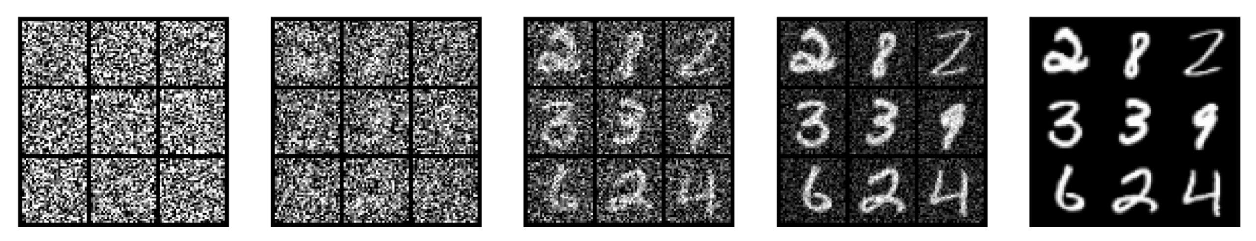
It is worth pausing on how nontrivial this is. No matter where you start, a protein structure, an image of a cat, a noisy sketch, applying small Gaussian perturbations enough times always lands you at the same easy-to-sample distribution: an isotropic Gaussian. The forward direction is universal. The generative problem reduces to inverting this “universal contraction”: if we can learn to undo the corruption step-by-step, we can sample new data points by starting at the Gaussian prior and reversing the chain.
A latent-variable view, and why we need a variational bound
Suppose we want to use the reverse direction to draw samples. We define a generative model that parameterises a reverse Markov chain,
where the prior matches the limiting marginal of the forward process, and each reverse transition is a Gaussian with parameters predicted by a neural network. To train, we want to maximise the likelihood of the observed data. Why the joint and not just directly? Because we cannot evaluate in closed form: it is the marginal of the joint over all intermediate states:
The integral on the right is over high-dimensional latent variables and is intractable. This is the standard situation in latent-variable models, and the standard fix, due to the VAE literature, is to lower-bound the log-likelihood with the evidence lower bound (ELBO). We introduce a variational distribution over the latents, multiply and divide by it inside the integral, and apply Jensen’s inequality to the resulting log of an expectation:
The expectation on the right is the evidence lower bound. Its negative is the variational lower bound loss,
which we minimise to push the model joint toward the data joint induced by .
What makes diffusion special compared to a generic VAE is that we fix the variational distribution to be the known forward process, not learnt, not parameterised, just the simple Gaussian chain we constructed above. This is the conceptual key: a diffusion model is a hierarchical VAE with latents whose encoder is frozen by design and whose decoder is a learnable reverse Markov chain.

The diagram above summarises the construction we have just walked through: a frozen forward Markov chain that destroys structure, and a learnable reverse chain that reconstructs it.
Decomposing
The integral defining is still high-dimensional, but it admits a clean per-step decomposition. Start by expanding the ratio inside the log, using the factorisations of and :
The forward conditionals are not directly comparable to the reverse conditionals : they go in opposite directions. To make them comparable, rewrite for using Bayes’ rule, conditioning everything on :
The first equality uses the Markov property of the forward chain; the second is Bayes. Substituting back and using a telescoping argument on the marginals (full derivation in [Ho et al., 2020, appendix A](#ref-ho2020)), one obtains
This decomposition has a beautiful structure. is essentially constant: it measures how close the forward marginal is to the prior , and is approximately zero by construction. is a final-step log-likelihood that becomes negligible at high . The interesting terms are the per-step KL divergences , which compare the true posterior , a Gaussian with closed form thanks to Bayes’ rule on Gaussians, against the model’s reverse conditional .
The true posterior is
with closed-form posterior mean and variance
Here we can notice how the new mean of the gaussian is an interpolation between the noisy state in which we are at point and the clean/unnoised sample at time zero!
From KL to MSE on means
A key fact, originally due to Feller (1949), is that when the forward step is Gaussian with sufficiently small variance , the exact reverse step is also approximately Gaussian. This is the formal justification for parameterising the model’s reverse conditional as a Gaussian with fixed covariance: with . The variance is fixed (not learned) to one of the two endpoints corresponding to the upper and lower bounds on the true reverse variance derived in Ho et al. (2020). The KL divergence between two Gaussians with the same covariance has a particularly simple form, it reduces to a scaled squared distance between the means:
So the entire per-step loss reduces to an MSE between the model’s predicted mean and the true posterior mean. The strategic question is then: how should we parameterise the network’s output to make this MSE easy to learn?
Using the reparameterisation , that is, expressing in terms of the noise that was used to construct , and substituting into , mechanical algebra gives
This suggests parameterising the model’s mean by the same expression but with a learnt in place of the true :
Substituting and into the KL expression and simplifying gives, after cancellation,
Each per-step VLB term has thus reduced to a weighted MSE between the true noise (drawn when we constructed ) and the network’s predicted noise. This is, structurally, vanilla supervised regression: predict given .
Ho et al. then made the empirical observation that dropping the time-dependent weight in front of this MSE produces strictly better samples than keeping the principled VLB weight. The resulting simple objective is the workhorse of modern diffusion:
The dropped weighting is largest for small (mild noise) and effectively upweights the harder high-noise levels, which empirically gives sharper samples (Ho et al., 2020).
This objective is extraordinarily efficient and scalable, and this is, in my view, the single most important reason diffusion models took off so quickly. Look at what training requires at each step: pick a data point from the training set, sample a timestep uniformly, sample a single Gaussian noise vector , form using precomputed tables, and regress with one network forward-backward pass. There is no need to simulate the trajectory. There is no MCMC inner loop, no ODE solver in training, no need to even store any state between iterations. The training cost per step is identical to that of a vanilla supervised regressor. This is the property that made diffusion scale from CIFAR-10 to ImageNet to text-conditional generation to protein design without much architectural rethinking.
Ancestral sampling
At inference time we want new samples from the trained model, so we must run the Markov chain backward. Start from and for apply the ancestral sampler:
We can observe here as well how the new less noisy sample at time is indeed our sample at time minus the noise that the networks recognizes in the sample. Heuristically, we are doing a step towards the denoised sample (away from the noise).
A later refinement worth flagging here: [Nichol & Dhariwal (2021)](#ref-nichol2021) showed that a cosine schedule,
avoids the pathology of the linear schedule destroying low-resolution signal too quickly; stays near 1 for longer in the early steps and then collapses smoothly. They also showed that learning a log-interpolation between and for the reverse covariance improves log-likelihood. Both choices are now standard.
DDPM in the wild: the original RFDiffusion sampler
The original RFDiffusion (Watson et al., 2023), one of the model that launched de-novo protein design as we know it today, is in this DDPM lineage. Its inner sampling loop in rfdiffusion/inference/utils.py implements exactly the ancestral update we have just derived. The key helper, get_mu_xt_x0, computes the posterior mean and posterior variance from cached and schedules:
def get_mu_xt_x0(xt, px0, t, beta_schedule, alphabar_schedule, eps=1e-6):
    """Given xt, predicted x0 and the timestep t, give mu of x(t-1)."""
    t_idx = t - 1
    # (1) Posterior variance: sigma = ((1 - alphabar_{t-1}) / (1 - alphabar_t)) * beta_t
    #     This is exactly tilde{beta}_t.
    sigma = (
        (1 - alphabar_schedule[t_idx - 1]) / (1 - alphabar_schedule[t_idx])
    ) * beta_schedule[t_idx]
    xt_ca  = xt[:, 1, :]    # C-alpha coordinates at time t
    px0_ca = px0[:, 1, :]   # network's prediction of clean C-alpha coordinates
    # (2) First term of the posterior mean: coefficient on x_0.
    a = (
        (torch.sqrt(alphabar_schedule[t_idx - 1] + eps) * beta_schedule[t_idx])
        / (1 - alphabar_schedule[t_idx])
    ) * px0_ca
    # (3) Second term of the posterior mean: coefficient on x_t,
    #     with sqrt(1 - beta_t) = sqrt(alpha_t).
    b = (
        (torch.sqrt(1 - beta_schedule[t_idx] + eps) * (1 - alphabar_schedule[t_idx - 1]))
        / (1 - alphabar_schedule[t_idx])
    ) * xt_ca
    mu = a + b
    return mu, sigma
And the helper that drives one ancestral step, get_next_ca, samples from the Gaussian in one line:
def get_next_ca(xt, px0, t, ..., noise_scale=1.0):
    # Compute posterior mean and variance from the cached schedules.
    mu, sigma = get_mu_xt_x0(xt, px0, t, beta_schedule, alphabar_schedule)
    # (4) Ancestral sampling: x_{t-1} ~ N(mu, sigma * I).
    sampled_crds = torch.normal(mu, torch.sqrt(sigma * noise_scale))
    delta = sampled_crds - xt[:, 1, :]
    ...
    out_crds = xt + delta[:, None, :]
    return out_crds / crd_scale, delta / crd_scale
Each numbered line is a line-for-line transcription of an equation from Section 1.
- Lines (1) is the closed-form DDPM posterior variance , with
alphabar_scheduleandbeta_scheduleprecomputed at startup. - Lines (2) and (3) are the two terms of the closed-form posterior mean
with written out as and replaced by the network’s predictionpx0(an -parameterisation rather than -parameterisation, but as we will see in Section 2 the two are linear transformations of each other in this Gaussians setting). - Line (4) is the ancestral sampling step itself: draw , exactly the per-step update from Section 1. The
noise_scaleknob is a protein-design-specific multiplier that lets the user trade off sample diversity against fidelity to the training distribution; settingnoise_scale = 1.0recovers the textbook DDPM sampler.
One little note to keep in mind here: RFDiffusion uses this Gaussian DDPM update only on the translational (C-alpha) part of the structure: rotations are diffused on with an IGSO(3) reverse process (the get_next_frames helper alongside get_next_ca in the same file), because the Gaussian formalism does not transfer cleanly to a curved manifold.
2. DDIM: Non-Markovian Generalisation and Deterministic Sampling
As mentioned above, the DDPM formulation allows for highly efficient training that can be parallelised and therefore scaled. At sampling time, however, the Markov structure of the process forces us to start from the tractable distribution at and traverse every step of the learned chain in reverse. This meant that even with a perfectly trained model one needed hundreds to thousands of network evaluations to produce a single sample. Song, Meng & Ermon (2021a) asked therefore the following question: does the DDPM training objective actually require the forward process to be Markov?
The answer is no, and the consequence is a sampler that converges in 20–50 steps instead of 1000.
A first observation: noise-prediction is denoised-image-prediction
Before deriving DDIM, it is worth absorbing the equivalence between two natural parameterisations of the network’s output. The forward marginal is
This is a linear relationship between three quantities (, , ). Given any two of them we can solve for the third:
So a network that takes as input and predicts is equivalent to a network that predicts : each prediction is a fixed linear transformation of the other (with coefficients that depend on but not on the data). In particular, if the network outputs we can immediately extract a denoised-image estimate
This is essentially the Tweedie-formula one-step denoiser: the network’s best guess of the clean image given the noisy observation. We will use it heavily in what follows.
Two equivalent ways to think about a denoising step. Both parameterisations describe exactly the same operation, but they invite different mental pictures.
- Predict the clean image, then take a small step toward it. Feed to the network and ask “what does the clean image look like?” Recall from the discussion of the true posterior mean above that one step of denoising is essentially an interpolation between the noisy state and the predicted clean state , with the interpolation weight controlled by the schedule. So a step of the reverse chain literally drags the sample a little closer to where the network thinks the data lives.
- Predict the noise, then subtract a small fraction of it. Equivalently, ask “what noise was added to produce ?” and remove a small portion of it, taking a step away from the noise direction. The two views are linked by the linear relation , so the two updates are mathematically identical.
The DDPM paper picked -prediction because the regression target has unit variance by construction (the network is asked to predict an vector at every ), which makes the network well-conditioned across the entire schedule. Different downstream methods will switch between parameterisations as convenient.
A family of non-Markovian forward processes
The DDPM loss depends only on the marginals : at each step we sample one from this marginal and regress. It does not depend on the joint in any way that involves the inter-step structure. Song et al. (2021a) leverage this: they consider an entire family of (possibly non-Markovian) forward processes that share the same per-step marginals as DDPM but differ in their posterior conditionals . Each member of this family corresponds to a valid sampler that re-uses the same trained noise predictor , no retraining needed.
The family is indexed by a sequence of stochasticity parameters and posits
The structure of this conditional is worth absorbing. The mean is a sum of two terms:
- : the signal component at noise level , i.e. where would project under the forward marginal at time ;
- : a scaled version of the noise direction implied by the pair .
Plus a Gaussian fluctuation of variance . Song et al. (2021a) prove that, for any choice of , this family yields the same marginals as DDPM, and therefore the same training objective and the same trained network are valid.
The DDIM sampler
Plugging in the network’s prediction in place of the true , we obtain the DDIM update in a very transparent form:
Compare directly with the DDPM ancestral update,
and the structural difference becomes clear. The DDPM update is a local perturbation of whose coefficients and are calibrated for a single Markov step — the step size is baked into the formula. The DDIM update instead reconstructs from scratch by combining the predicted clean image (rescaled to the target noise level via ) with the predicted noise direction (rescaled by ). The target time index enters the right-hand side only through the cumulative noise level ; the local step quantities and do not appear explicitly at all. (The source time still enters, of course, through and , which depend on and .)
The stochasticity parameter is conventionally written
with interpolating between two limits:
- recovers the DDPM ancestral sampler (up to a covariance choice equivalent to );
- gives the deterministic DDIM sampler, the workhorse of the modern fast-sampling regime:
Why DDIM allows fewer sampling steps
It is tempting to attribute DDIM’s step-skipping ability simply to “the trajectory is smooth.” That is part of the story but not the whole picture. Three observations, each with a clean intuitive content, together explain the effect.
(i) The update is anchored to a noise-level-agnostic prediction. Look again at the DDIM update: the right-hand side combines (the network’s guess of the clean image) and (the noise it sees) with coefficients and for any target noise level — and in the deterministic () case, this collapses to the clean form and displayed above. Crucially, does not depend on which we want to jump to, it just depends on the current . So once the network has produced its best guess of the clean image, the formula can reassemble a sample at any lower noise level by simply remixing signal and noise in the proportions appropriate to that level. We can leap directly from to without visiting any intermediate state. (Song et al. formalise this in Section 4.2 / Appendix C.1 of the paper: the same update applies along any sub-sequence , replacing with .) Contrast this with the DDPM update, whose right-hand side contains . That coefficient encodes the size of a single small Markov step: it tells the sampler how much progress to make in one increment. There is no analogous “leap to ” knob, because the DDPM step size is hard-coded into the formula itself.
(ii) DDIM is a first-order discretisation of an ODE, not an SDE. In the deterministic case there is no fresh noise injection at each step, so the only source of error is the truncation error of the ODE solver, i.e. the discrepancy between the discrete update and the continuous probability-flow trajectory we will discuss in Section 3. Truncation error scales smoothly with step size and accumulates additively. SDE discretisations are different: each step injects fresh Gaussian noise whose variance scales with the step size, so larger SDE steps mean noisier samples in a way that no amount of network accuracy can fix. ODE solvers do not suffer from this.
(iii) The probability-flow trajectories tend to be relatively low-curvature. Karras et al. (2022) later showed empirically that the deterministic trajectory from prior to data in diffusion models is approximately linear over much of its length, with most of the curvature concentrated near the data manifold. A nearly-straight trajectory is well-approximated by a few large Euler steps.
Together these three points explain the empirical observation that DDIM with 20–50 steps matches DDPM with 1000 steps at no cost to model retraining. DDIM also gives an invertible encoding from noise to data, which is the substrate of latent-space interpolation, editing, and exact likelihood evaluation via the change-of-variables formula.
Intuition: DDIM keeps the same marginals as DDPM but parameterises the reverse process around , the predicted clean image, rather than around . Each step says “given my best guess of the clean image, where would I be at noise level ?” This is invariant to step size: the formula is happy to jump to any target noise level. Removing the stochasticity () on top of this turns sampling into a deterministic trajectory you can traverse with bigger strides.
3. Score-Based Generative Modelling Through SDEs
A few months after DDIM, [Song, Sohl-Dickstein, Kingma, Kumar, Ermon & Poole (2021b)](#ref-song2021b) published the paper that, in retrospect, unified everything that came before. Two parallel threads had been developing in the literature:
- The DDPM thread I described above, descending from variational hierarchical-VAE constructions and trained with the -prediction MSE.
- The NCSN / SMLD thread initiated by [Song & Ermon (2019)](#ref-songermon2019), “Noise Conditional Score Network” and “Score Matching with Langevin Dynamics”, which trained a network to estimate the score function of a noise-corrupted version of the data distribution at many noise scales . To sample, NCSN ran annealed Langevin dynamics: starting from a wide Gaussian, take some Langevin steps at the largest , anneal to the next smaller , repeat.
The training objective for NCSN was denoising score matching (Hyvärinen, 2005; Vincent, 2011), and the sampler was a discrete-time Langevin chain. Song et al. (2021b) showed that both DDPM and NCSN are discretisations of the same continuous-time stochastic differential equation. This unification opened the door to better samplers, exact likelihood evaluation via the probability-flow ODE, and a host of downstream methods including guidance and inverse-problem solvers.


Forward SDE: setup and three regimes
The forward corruption is now an Itô stochastic differential equation on :
where is a standard -dimensional Wiener process (Brownian motion), is the drift coefficient, and is the diffusion coefficient. Three concrete choices of recover existing models:
(a) Variance Preserving (VP-SDE), the continuous-time limit of DDPM:
This is an inhomogeneous Ornstein–Uhlenbeck (OU) process: a stochastic process whose drift is a linear restoring force pulling toward the origin (with strength ), and whose diffusion term injects isotropic noise (of strength ). The “pull toward the origin” can be read directly off the drift coefficient : it always points in the direction opposite to the current state , with magnitude proportional to the distance from the origin. So if sits far out along some axis, the deterministic part of the dynamics pushes it back toward zero; if is already near the origin, the drift is small. This is the continuous-time analogue of the discrete forward step from Section 1, where the factor was shrinking the mean toward zero at each step. The asymptotic stationary distribution as is , the Gaussian prior we want.
(b) Variance Exploding (VE-SDE), the continuous-time limit of NCSN / SMLD:
Notice: no drift. The data is never rescaled; only noise is added, at a rate determined by the schedule . The marginal is , and as the marginal becomes a very wide Gaussian centred at : the variance literally explodes. The oppposite process will therefore look like a “huge gaussian collapsing” into a new generated sample
(c) sub-VP-SDE, introduced in the same paper:
This is a hybrid with variance strictly less than the VP-SDE at every , empirically giving better likelihoods on CIFAR-10. We will not dwell on it but it’s worth knowing it exists.

DDPM is a discretisation of the VP-SDE
The claim that DDPM is the VP-SDE in disguise is worth working out, because the algebra is short and clarifying. Discretise the VP-SDE with the Euler–Maruyama scheme, the simplest first-order numerical scheme for SDEs, using a step :
so
Now identify the discrete DDPM coefficients with the continuous SDE coefficients via (i.e. the discrete in DDPM is times the time-step). For small we have the Taylor expansion , so
The Euler–Maruyama discretisation thus reads
which is exactly the DDPM forward step from Section 1. So DDPM is literally the Euler–Maruyama discretisation of the VP-SDE with .
Why is VP-SDE “variance preserving”?
Take the scalar case for clarity and compute the conditional variance recursively. From the forward step with independent of :
If , then . So once the variance reaches one, it stays exactly one, independently of the schedule . This is the precise sense in which the VP-SDE preserves variance: the marginal variance is a fixed point of the forward dynamics at value 1. The forward process keeps every in roughly the same magnitude range as the data, which is convenient numerically.
How VE-SDE is the continuous limit of NCSN/SMLD
Now to the variance-exploding side. NCSN/SMLD as originally constructed (Song & Ermon, 2019) trains a network at discrete noise scales : at scale the “data” is , with drawn from the dataset. The network outputs an estimate of the score at each scale, where denotes the data distribution convolved with .
To pass to the continuous-time version, let the discrete scales become a continuous schedule and ask: which SDE produces marginals where ?
Since the marginal mean is (constant in ), the drift must be zero: . The marginal variance is , and for an SDE with zero drift and diffusion , the variance evolves as
Setting gives , hence
This is exactly the VE-SDE coefficient. The corresponding SDE is
with marginal , exactly the family of noise-corrupted distributions that NCSN trains on. So VE-SDE is the continuous schedule limit of NCSN’s discrete noise-scale construction: in the same way DDPM is the continuous limit of VP, NCSN is the continuous limit of VE.
The term “variance exploding” refers to the divergence of at large : in standard NCSN setups is geometric with in the dozens or hundreds, so the marginal at late time has variance much greater than 1. In contrast, VP keeps variance bounded at 1.
Numerical example (VP vs VE at matched SNR)
The cleanest way to see the geometric difference between VP and VE is to match them at the same signal-to-noise ratio (SNR). For each, with :
Setting these equal gives the conversion . Picking three noise levels and applying the same , :
| Noise level (SNR) | under VP | under VE | VP | VE | ||
|---|---|---|---|---|---|---|
| Low (SNR=9) | 0.9 | 0.333 | 0.10 | 0.111 | ||
| Mid (SNR=1) | 0.5 | 1.000 | 0.50 | 1.000 | ||
| High (SNR=1/9) | 0.1 | 3.000 | 0.90 | 9.000 |
Reading the table left-to-right: at every row, VP and VE encode the same amount of information about (same SNR), but they live on completely different scales. VP keeps the magnitude of bounded near 1 across all noise levels. VE lets the magnitude grow without bound, at high noise the data is a vanishing perturbation of a wide Gaussian. Same , same information content, drastically different geometry.
Reverse-time SDE and the score function
The fundamental theoretical result of Song et al. (2021b) is the reversibility of the forward SDE. Due to Anderson (1982), every Itô diffusion admits a reverse-time companion whose drift is the original drift minus the score of the time-marginal:
where is a reverse-time Brownian motion. If we can estimate the score at every (call this estimate ), we can simulate the reverse-time SDE numerically (Euler–Maruyama again) and produce a sample from starting from .
The score is learned by denoising score matching (Vincent, 2011). The loss is
Because is a Gaussian with closed form, the conditional score is analytic. For VP at time , , so
This is the exact mathematical bridge to DDPM: predicting the noise and predicting the score are the same regression problem up to a fixed scalar . The DDPM simple loss and the NCSN denoising score matching loss differ only in the constant in front of the MSE, which is absorbed into the weighting function .
Probability-flow ODE: same marginals, no noise
A deep observation from Song et al. (2021b): the family of stochastic processes that share the same marginals as the reverse SDE is not unique. There is a privileged deterministic member, the probability-flow ODE:
Solving this ODE backward in time from to produces a sample with the same marginal distribution at every as the reverse SDE, but along a deterministic, invertible trajectory. The probability-flow ODE:
- underlies DDIM, which is (up to a notational change) its first-order Euler discretisation in the VP regime;
- enables exact log-likelihoods through the instantaneous change-of-variables formula ;
- is the substrate on which EDM will later build.
Intuition (score as force). The score is the gradient of the log-density: it points uphill in , toward higher-density regions, i.e. toward the data manifold. In the reverse SDE, the term in the drift is therefore an attractive force pulling the sample toward the data manifold. The Brownian term is exploratory: it injects random fluctuations that prevent the sample from collapsing onto any particular trajectory. The balance between these two, attraction toward data versus stochastic exploration, is exactly the exploration–exploitation tradeoff familiar from Langevin MCMC and from many sampling algorithms in statistical physics. The probability-flow ODE keeps the attraction and drops the exploration entirely, giving a deterministic trajectory that is the “expected” reverse path.
Predictor–corrector sampling and Langevin correctors
A practical contribution of Song et al. (2021b) that I find under-appreciated is predictor–corrector (PC) sampling. The motivation is that any numerical SDE solver makes errors at each step: the discretised sample at time has a distribution that drifts from the true marginal . Over many steps these errors compound. The idea of PC is to correct the sample’s distribution back onto the true after each predictor step by running a small number of MCMC steps targeting , using the same learnt score we already have.
The corrector of choice is Langevin MCMC (a.k.a. unadjusted Langevin algorithm or ULA). To sample from a density , Langevin dynamics is the SDE
Its stationary distribution is . Discretising with the Euler–Maruyama scheme and a step size ,
Here is the Langevin step size, a hyperparameter that controls how aggressively the corrector moves toward higher-density regions per Langevin step. (It is not the SDE timestep , it is the discretisation parameter of a different SDE that runs at fixed outer time.) A typical PC sampling iteration looks like:
- Predictor: One reverse-SDE step from at time to at time (e.g. Euler–Maruyama with the learnt score).
- Corrector: Langevin steps at fixed time targeting :
The number of Langevin steps and the step size are tuned per problem; Song et al. (2021b) typically use and a small , choosing it so that the “signal-to-noise ratio” of the Langevin update matches a target value. PC samplers gave a noticeable quality boost over plain Euler–Maruyama at the same total number of function evaluations, and the principle, interleave deterministic transport with score-driven stochastic correction, reappears in EDM’s stochastic sampler.
Why this looks familiar to anyone who has run a molecular dynamics simulation. Langevin dynamics is exactly the equation of motion used in MD with a stochastic thermostat: under the identification (with a potential energy and a temperature), the term becomes the negative gradient of a potential, i.e. a force. So the Langevin step
reads, in MD language, as “take a small step in the direction of the force, and add a thermal kick.” Just as MD with a Langevin thermostat samples the Boltzmann distribution at long times, our corrector samples the target distribution at long times. The score played by the neural network is, by analogy, a learnt force field: a position-dependent vector field whose flow lines lead the sampler toward high-density regions of . The thermal noise prevents the sample from collapsing into a single energy minimum (a single mode of ), exactly as it does in MD at finite temperature. This is a useful mental picture when you want to reason about ergodicity, mode mixing, or step-size choices in the sampler: most of the intuition built up in computational statistical mechanics transfers directly.
4. EDM: Elucidating (and Simplifying) the Design Space
By 2022 the diffusion literature had accumulated a small zoo of choices (VP vs VE, – vs score- vs -prediction, linear vs cosine schedule, ancestral vs DDIM vs PC) and it was not clear which combinations mattered for sample quality and which were essentially cosmetic. Karras, Aittala, Aila & Laine (2022), in “Elucidating the Design Space of Diffusion-Based Generative Models” (EDM), attacked this head-on by re-deriving everything in a single, opinionated parameterisation and then ablating each design choice independently. The result is what has become the default in modern image-diffusion and protein-diffusion codebases.
Source. The exposition of the EDM sampler in this section follows closely the excellent talk by the EDM authors on the design space of diffusion samplers. I highly recommend watching it in full: it is the clearest single source I know of for the geometric intuition behind the -parameterisation, preconditioning, and Heun-plus-churn sampling.
The “x-ray view”: decoupling the design choices
The framing the EDM authors themselves use is worth absorbing. Before EDM, methods like VP, VE, iDDPM, and DDIM looked like tightly coupled packages you had to take as a whole: you couldn’t, say, combine the iDDPM noise schedule with the DDIM sampler without something breaking, because each package’s choices were implicitly tangled. EDM gives an x-ray view into the internals: it shows that any such method decomposes into a small set of orthogonal design choices,
- the ODE / SDE solver (Euler, Heun, RK45, …),
- the time-step discretisation (where to place the sampling points along ),
- the noise schedule (how grows with the abstract time variable),
- the signal scaling (whether and how is rescaled),
- the network preconditioning (),
- the training noise distribution ,
- the loss weighting ,
each of which can be tuned in isolation, without retraining the network and without affecting the validity of the other choices. Armed with this decomposition, Karras et al. systematically searched for the best individual setting of each axis and stacked the improvements.
Sampling and training can be mixed and matched freely. An immediately useful practical consequence of the decoupling above: the training-time choices (preconditioning, loss weighting, noise distribution) and the sampling-time choices (solver, time-step schedule, churn) live on independent axes. You can take a network trained with the iDDPM noise distribution and weighting, and run it with the EDM Heun sampler at inference, no retraining required. Indeed, much of the empirical force of the EDM paper comes from precisely this experiment: Karras et al. apply their improved sampler to off-the-shelf pre-trained VP, VE, and iDDPM models and obtain large quality gains without touching the weights. The corollary is that sampler design and training design can be iterated on independently, a huge practical win, because re-training a diffusion model is expensive while changing the sampler is essentially free.
Before going through their choices it helps to name the two distinct error sources in sampling, which we want to analyse in isolation:
- Network (denoiser) error: even if numerical integration were exact, the denoiser is only an approximation of the optimal denoiser, so it pushes the trajectory in a slightly wrong direction at each step.
- Truncation error: the deterministic trajectory we want to integrate is a curve in -space, and any solver discretises it with straight segments. Larger steps mean larger curvature-induced deviations from the true curve.
These two sources interact (worse network → larger drift → harder for the solver), but the sampler design controls primarily the second, while the training design controls primarily the first. EDM separates them cleanly.
The -parameterisation
EDM throws out the discrete time index and works directly with the noise level . The forward path is the simplest possible:
i.e. a variance-exploding path with playing both the role of “time” and “noise scale.” Karras et al. pick so that and no signal-scaling is applied. Their justification, which I think is the single deepest insight of the paper, is given in the next subsection.
Two ways to deal with the signal-magnitude problem
A practical concern with the VE path is that for large , the magnitude of becomes huge, values in the tens or hundreds, well outside the comfortable unit-scale range that neural networks like to operate in. Naively feeding at to a CNN is asking for unstable training.
There are exactly two principled cures for this, and they correspond to the two camps in the pre-EDM literature:
Cure 1 (VP-style): rescale the signal inside the forward path. Introduce an explicit signal scaling so that the actual sample fed to the network is , with chosen to keep the magnitude of bounded. This is what VP does implicitly: setting is exactly a rescaled version of the VE path, with squeezing the signal down to keep total variance at 1.
Cure 2 (VE + network preconditioning): leave the path alone, rescale at the network’s input and output. Keep the simple VE path in its raw form, but wrap the neural network so that its input is divided by (giving unit-variance input) and its output is multiplied by an appropriate -dependent factor. From the network’s point of view it always sees well-scaled tensors, even though the underlying ODE state may have huge magnitude.
Both cures solve the same numerical problem and let the network see well-scaled tensors throughout training and sampling. But they have very different geometric consequences for the underlying ODE trajectory. The VP rescaling distorts the natural flow lines of the ODE: it bends what would be a near-linear trajectory in -space into a curved one. The VE-plus-preconditioning approach leaves the ODE alone (the flow lines retain whatever natural geometry they have) and absorbs the multi-scale problem inside the network. EDM argues, and demonstrates empirically, that the second cure is strictly better: straighter flow lines mean fewer Euler steps are needed for the same quality. This is why EDM commits to (no signal scaling in the ODE) and pushes all the magnitude management into preconditioning.
Deriving the EDM ODE from the forward path
The probability-flow ODE for a general SDE was given in Section 3. For the VE-SDE with and it becomes
Now invoke Tweedie’s formula: for with ,
equivalently , where is the optimal MMSE denoiser. MMSE stands for minimum mean squared error: among all measurable functions predicting from a noisy observation , the conditional expectation is the unique minimiser of the expected squared error . So is precisely the object that a network trained with an MSE loss would converge to in the infinite-data limit: predict the clean image given the noisy one. Tweedie’s formula tells us this denoiser and the score are two views of the same underlying quantity.
Substituting the Tweedie expression and using so that :
This is the EDM ODE, the most economical form one can write for the deterministic generative dynamics. The sign convention deserves a careful word, because at first glance the formula looks like it points the wrong way.
First, a clarification that is worth being explicit about. The forward noising introduced at the start of this section, , is the marginal of the stochastic VE-SDE . The equation we just derived is a different equation: it is the probability-flow ODE, a deterministic dynamical system whose only relation to the noising SDE is that it shares the same marginal distributions at each noise level. They are not the same trajectory and not the same equation; they only agree on the one-time marginals.
The defining property of the PF-ODE, stated explicitly by Karras et al. (2022) (Section 2), is that integrating it from to — either forward or backward in — produces a sample distributed according to the marginal . Because the PF-ODE is deterministic, its solutions can be traversed in either direction of , and Karras et al. give the intuition in two complementary sentences: “an infinitesimal forward step of this ODE nudges the sample away from the data… equivalently, a backward step nudges the sample towards the data distribution.” So the same PF-ODE can be used either to corrupt (integrate with , toward larger noise) or to generate (integrate with , toward smaller noise).
Now interpret the formula in each direction. Read with increasing (increasing noise level ), the velocity vector points in the direction , i.e. away from the denoiser’s estimate of the clean image — consistent with the corruption story (sample drifts away from the data manifold as grows). To generate samples we integrate with , so a single Euler step is , which is a step in the direction , toward the current best guess of the clean image. The sampler does the intuitive thing.
The apparent singularity at also deserves a closer look. The numerator and the denominator both vanish: as the optimal denoiser becomes the identity (), so . The two zeros race each other and the resulting limit is finite. To see this concretely, expand to first order in : for small , (this is just Tweedie’s formula again, rearranged), so
The velocity therefore vanishes as , and the trajectory smoothly settles onto the data manifold rather than blowing up.
The tangent points directly to the denoiser output: why this matters. Suppose at time we extrapolate a single linear Euler step from all the way down to . Plugging into ,
So with the schedule, the tangent direction points exactly to the current denoiser output. This is not true for other schedules: for VP, or for any choice with signal-rescaling , the tangent points to some weird intermediate target that depends on the schedule’s curvature. Empirically, the denoiser output , the model’s best guess of the clean image, changes very slowly along the sampling trajectory. Once you have an approximately right guess of the clean image, that guess remains approximately right as you anneal downward. So the tangent direction is roughly constant across steps, which is exactly the condition under which large Euler steps work well. This is the deepest answer to “why does DDIM-style ODE sampling take such big strides?”: the dynamics really want this schedule.
Preconditioning: deriving the EDM coefficients
The single most empirically impactful contribution of EDM is the explicit preconditioning of the network. Rather than asking a raw network to output or across many orders of magnitude of , Karras et al. write
and derive the coefficients analytically from two simple desiderata: the network’s input should have unit variance, and the network’s training target should have unit variance. Let me walk through the derivation.
Assume has variance per coordinate (typically for normalised images). Then has variance . For the network’s input to have unit variance,
The training loss is . Substituting the preconditioned form and rearranging, the network’s effective target is
We want . Expanding the numerator,
with variance . To minimise the magnitude of this target across , equivalently, to give the network the least extreme regression problem, we choose to minimise this variance. Setting the derivative with respect to to zero:
Substituting back, the residual variance is
For unit variance of the network target we need , hence
Finally, is the input embedding of the noise level, for which Karras et al. use the heuristic .
Why this matters in practice: the two extremes. The behaviour of these coefficients at small and large explains why preconditioning is empirically transformative.
- At small (clean image, ): and . The architecture essentially copies the input through the skip, and the network’s output is a small correction scaled down by . If the network makes an error, that error is multiplied by a small number on its way out, downscaled, not amplified. The network is freed from having to learn the identity function (a real risk in naive setups) and can focus on producing a small denoising correction.
- At large (mostly noise, ): and . The skip is effectively disabled, and the network is asked to predict the clean signal directly. This avoids the disaster of a naive noise-prediction setup, where the network would predict and have its output multiplied by , meaning a network error of order becomes an output error of order , amplified by a potentially huge factor when is in the dozens.
The analytic smoothly interpolates between these two regimes, automatically selecting “predict residual / predict signal” depending on how noisy the input is. The transition happens around . The neural network always sees well-scaled inputs and produces well-scaled outputs; the brunt of the multi-scale problem is absorbed by an analytic skip connection.
A further upside the EDM authors emphasise: because the preconditioning analytically handles the scale variation, the architecture of the inner network is now essentially free to be whatever you want (DDPM-style U-Net, NCSN-style, transformer, etc.) and the preconditioning works for “any” architecture. EDM cleanly separates “what the network is” from “how its inputs and outputs are scaled.”

The EDM sampler: Heun with stochastic churn
For sampling, EDM proposes a deterministic and a stochastic variant of the same core procedure. The deterministic version is Heun’s second-order ODE solver applied to the EDM ODE: for each step from to ,
Heun is a predictor–corrector scheme in the numerical-analysis sense: take a tentative Euler step, evaluate the slope at the predicted endpoint, then re-step using the average of the two slopes. The second-order trapezoidal correction halves the truncation error per step compared to plain Euler (or first-order DDIM) at the cost of one extra denoiser evaluation per step. Karras et al. tested various higher-order solvers (RK45, linear multistep methods) and reported that Heun strikes the best quality-per-NFE tradeoff.
The stochastic variant adds Langevin-style churn: at the start of each step, inflate the current sample’s noise level by a small factor, then take a deterministic Heun step from the inflated level back down to . Concretely:
followed by a Heun step from to . The hyperparameters control how much, where in the schedule, and with what amplification noise is reinjected. The interpretation is exactly the predictor–corrector logic from Section 3 in a different disguise: the noise injection is the “Langevin exploration” that washes out deterministic drift error; the Heun step is the deterministic transport that follows the ODE flow lines. Putting them together at each step is empirically more controllable than running a full reverse-SDE solver.
The Karras -schedule: spend more steps near the data
The noise levels themselves are not linear or geometric but follow a power law parameterised by :
The defaults , , , and allocate disproportionately many steps to the low- end, where the sample is close to the denoised image. The motivation is twofold:
- Close to the data manifold, the ODE trajectory has its highest curvature. Far from the data the dynamics are gentle and approximately linear (recall that the EDM tangent points to the denoiser output, which barely changes). Close to the data the trajectory “locks onto” a specific sample, and the denoiser output begins to commit to fine details; this is where the flow lines turn. Linear Euler steps are most error-prone in regions of high curvature, so we want fine resolution there.
- Small errors near the data are perceptually catastrophic. An error of magnitude at small produces a visible artifact in the final sample (low means is almost the final image, and any deviation will appear in the output as-is). The same error at large gets washed out by subsequent denoising. Putting more steps where they matter gives much better quality per NFE.
Increasing makes the allocation more lopsided toward small . The default was found by ablation; “Karras sigmas” with this schedule are now the default in essentially every modern image-diffusion pipeline.

Training: loss weighting and the noise level distribution
EDM’s training prescription is short but important enough that it deserves explicit treatment. Two choices complement the architectural preconditioning.
The noise level distribution during training is log-normal:
The motivation here is the mirror image of the sampling-schedule argument above. Empirically, the per- training loss has a roughly U-shape: at very low (the input is almost clean) the denoising task is trivial (any reasonable network produces a near-identity mapping) and there is little gradient signal to learn from. At very high (the input is mostly noise) the denoising task is essentially hopeless (no signal to recover) and gradients are again uninformative. The sweet spot, where the network can actually make progress and gradients carry real information, sits in the middle of the range. The log-normal distribution above concentrates training samples in exactly this regime, putting computational effort where the model can actually learn something.
Note that the sampling and training schedules answer different questions. Sampling allocates more steps near small because that is where truncation error is most damaging. Training allocates more samples near intermediate because that is where gradient information is richest. The two need not coincide, and in EDM they don’t.
The loss weighting that complements this is
This is chosen to equalise the gradient magnitude across noise levels. Without proper weighting, a naive loss has gradients that vary by orders of magnitude across , leading to highly imbalanced training: most updates push the network gently while occasional high-magnitude updates dominate. The weighting , combined with the unit-variance preconditioning, produces gradient updates of comparable magnitude at every , which empirically gives much more stable training dynamics.

An important observation on stochasticity, paraphrased from the EDM authors’ talk. The stochastic-churn sampler is empirically helpful, but it is a double-edged sword. The Langevin churn introduces its own discretisation error on top of the deterministic Heun step, so the net benefit depends on a delicate balance, and the optimal churn hyperparameters need to be tuned per dataset and per architecture, with no clean principles for how to do this. Worse, churn can mask bugs and modelling errors: a model with a slight bias in its denoiser can still produce reasonable samples under enough exploration, even when its deterministic samples reveal that something is wrong.
The authors’ recommendation, which I have come to follow in my own protein-design work, is: develop and debug in fully deterministic mode (Heun on the PF-ODE), and add stochasticity as “the final cherry on top” only after you are confident the deterministic samples look right. As a calibration point, the EDM CIFAR-10 model benefits negligibly from churn at its trained quality (the network is good enough that any exploration injects more error than it fixes), while their ImageNet-64 model still benefits, a useful empirical pointer that the marginal value of churn diminishes as the score network gets better.
EDM in the wild: the RFDiffusion3 inference sampler
To make the relevance of all this concrete, let us look at how the state-of-the-art protein-structure generator RFDiffusion3 implements its sampler. The relevant code lives in inference_sampler.py in the RosettaCommons foundry repository, in a method tellingly named sample_diffusion_like_af3. Stripping out the protein-specific bookkeeping (motif handling, classifier-free guidance, recycling, logging), the inner loop is essentially this:
for step_num, (c_t_minus_1, c_t) in enumerate(zip(noise_schedule, noise_schedule[1:])):

    # (1) Stochastic churn: inflate the current noise level by (1 + gamma).
    gamma = self.gamma_0 if c_t > self.gamma_min else 0
    t_hat = c_t_minus_1 * (gamma + 1)

    # (2) Inject noise to match the inflated level: epsilon ~ sqrt(t_hat^2 - t^2) * z.
    epsilon_L = (
        self.noise_scale
        * torch.sqrt(torch.square(t_hat) - torch.square(c_t_minus_1))
        * torch.normal(mean=0.0, std=1.0, size=X_L.shape, device=X_L.device)
    )
    X_noisy_L = X_L + epsilon_L

    # (3) Call the preconditioned denoiser D_theta(x; t_hat) on the inflated state.
    X_denoised_L = diffusion_module(X_noisy_L=X_noisy_L, t=t_hat.tile(D), ...)

    # (4) EDM tangent direction: (x - D(x; t_hat)) / t_hat.
    delta_L = (X_noisy_L - X_denoised_L) / t_hat   # "gradient of x wrt. t at x_t_hat"
    d_t = c_t - t_hat

    # (5) First-order Euler step along the EDM ODE.
    X_L = X_noisy_L + step_scale * d_t * delta_L
Each of these five lines is a line-for-line transcription of an equation we have just derived.
- Lines (1) and (2) are EDM’s stochastic churn: followed by . The thresholding if else is exactly the
S_min/S_maxwindow from the EDM paper, deciding where in the schedule to spend the churn budget. - Line (3) is the call to the preconditioned denoiser . The
diffusion_modulehere wraps the inner network with the analytic skip-connection and input/output scalings we derived above. - Line (4) is literally the EDM ODE: . The variable is even named
delta_Land the comment in the source code reads “gradient of x wrt. t at x_t_hat”. - Line (5) is the Euler step , with an extra
step_scaleknob that lets the user dial the step magnitude up or down (useful for trading sample diversity against fidelity in protein design).
Two small caveats worth flagging. First, RFDiffusion3 uses a first-order Euler integrator rather than the second-order Heun method recommended in the EDM paper; in practice the protein community has found that the extra denoiser evaluation per step is not worth its cost when the network is already expensive. Second, the step_scale and noise_scale multipliers are protein-design-specific knobs grafted on top of the pure EDM recipe to control downstream metrics like RMSD-to-motif and sample diversity, the kind of practical adjustment one always finds when transplanting a recipe from images to structures.
The point is that essentially every line of the inner sampling loop of a modern de-novo protein-design model is exactly the Karras et al. EDM sampler from Section 4, with the same churn, the same tangent direction, and the same preconditioned denoiser at its heart. Everything we have built up in this section is not retrospective taxonomy: it is the code path running every time someone designs a new protein with RFDiffusion3.
5. The Variance Schedule, Up Close
Because every method we have discussed is, mathematically, a particular Gaussian probability path , it is worth pausing to lay out side by side the choices of that constitute the variance schedule in each framework.
| Framework | (when ) | Boundary at | ||
|---|---|---|---|---|
| DDPM / VP, linear | , linear | (preserved) | ||
| DDPM / VP, cosine | (preserved) | |||
| NCSN / VE | , geometric or polynomial | (exploding) | ||
| sub-VP | (note: no square root) | at intermediate | ||
| EDM | via power law | (VE-like) | truncated at , not |
A few comments worth internalising. Linear vs cosine is a small but consequential change: Nichol & Dhariwal (2021) noted that the linear schedule destroys the signal far too aggressively in the early-to-middle timesteps for low-resolution images, leaving the network nothing to learn during the late part of training; the cosine schedule keeps near 1 for longer and then collapses smoothly. VP vs VE is a more fundamental geometric choice: under VP the trajectory stays inside a unit ball, under VE it expands outward. EDM is essentially VE plus principled preconditioning, which restores numerical stability and lets the network see well-scaled inputs at every . Finally, sub-VP sacrifices a small amount of sample quality for a sharper concentration around at intermediate , improving likelihood.
6. Connections, Tradeoffs, and Where the Field Sits
It is now possible to draw the picture cleanly. Every method we have discussed corresponds to a choice of three things:
- A probability path interpolating noise and data, defined by . VP, VE, sub-VP, and EDM-VE are different paths.
- A regression target (, , or score ), all of which are related by exact closed-form linear transformations once the path and prior are fixed.
- A sampler, either an SDE solver (DDPM ancestral, reverse-SDE Euler–Maruyama, EDM-stochastic), a deterministic ODE solver (DDIM, Heun, RK4), or a hybrid (predictor–corrector, EDM-churn).
The historical narrative is essentially that successive papers separated these three choices and showed that mixing them productively gives better samples. DDPM coupled VP, -prediction, and ancestral SDE sampling. DDIM kept VP and but swapped the sampler for an ODE. Song et al. (2021b) showed all of these are discretisations of a continuous SDE and that the same model admits both stochastic and deterministic samplers, and introduced VE and sub-VP. EDM then showed that with the right preconditioning and ODE solver, the difference between VP and VE essentially vanishes and most empirical gains come from sampler quality and noise-level distribution at training.
The stochastic vs deterministic tradeoff is worth spelling out. Stochastic samplers (DDPM, reverse-SDE, EDM with churn) act as their own error correctors: noise injection at intermediate steps washes out accumulated drift error from the score network, often producing better FID at high NFE than the corresponding deterministic ODE solver on the same model. Deterministic samplers (DDIM, Heun on the PF-ODE) are faster per quality at low NFE, are invertible (useful for editing, latent interpolation, likelihood evaluation), and are reproducible. Karras et al. (2022) systematically characterise this crossover; in my own protein-design work I tend to use the deterministic Heun sampler for NFE budgets under ~30 and switch to stochastic-churn variants when I have NFE to spare or am worried about mode coverage.
Comparison of sampling methods
| Method | Year | Key idea | Sampling type | Pros | When to use |
|---|---|---|---|---|---|
| DDPM (Ho et al.) | 2020 | Reverse Markov chain, -prediction, linear | Stochastic (ancestral) | Simple, foundational, robust training | Reference implementations; teaching |
| DDIM (Song et al.) | 2021 | Non-Markovian forward, deterministic | Deterministic (or interpolated) | 10 to 50 times fewer steps than DDPM, invertible, latent interpolation | Fast inference with an existing DDPM-trained model |
| NCSN / VE-SDE (Song & Ermon; Song et al.) | 2019 / 2021 | Score matching at multiple noise scales; Langevin sampling | Stochastic (Langevin / SDE) | Strong likelihoods; PF-ODE for exact density | High-noise regimes; likelihood-critical applications |
| VP-SDE / sub-VP (Song et al.) | 2021 | Continuous-time DDPM via SDE; PC sampler; PF-ODE | Both | Unified framework; principled likelihood; PC samplers | When you want the SDE formalism (e.g. inverse problems, guidance) |
| EDM (Karras et al.) | 2022 | -parameterisation, preconditioning, Heun + churn | Both | Best FID per NFE; clean code; modular | Modern default for image / structure diffusion; my default in protein work |
The current state of the art in protein-structure generation is, at the time of writing in May 2026, a mixture of these ingredients. Backbone-generation models like RFDiffusion descend directly from the score-SDE / EDM lineage. The point I would press on a student starting the field now is that the training objectives across all of these are nearly identical regression losses on linear reparameterisations of the same quantity (noise, clean data, or score), and what really differs between methods is the path, the sampler, and the symmetry group baked into the network. Pick the path that gives the geometry you want; pick the sampler that matches your NFE budget; train the same kind of MSE in every case.
Where to look next
The story above stops short of an important and very active branch of the field: flow matching and its relatives (rectified flow, OT-CFM). These methods drop the diffusion construction entirely and learn the velocity field of an ODE that transports noise to data along arbitrary, often straight-line, probability paths. They have become dominant in protein-structure generation since roughly 2023 and deserve their own dedicated treatment. For a broader and excellent overview of this family I recommend the MIT 6.S979 lecture notes on diffusion and flow-based generative models, which cover flow matching, conditional flow matching, and the connections back to the score-based picture we have built up here.
References
- Anderson, B. D. O. (1982). Reverse-time diffusion equation models. Stochastic Processes and Their Applications 12(3), 313–326.
- Feller, W. (1949). On the theory of stochastic processes, with particular reference to applications. Proceedings of the (First) Berkeley Symposium on Mathematical Statistics and Probability, 403–432.
- Ho, J., Jain, A., & Abbeel, P. (2020). Denoising Diffusion Probabilistic Models. NeurIPS 2020. arXiv:2006.11239.
- Hyvärinen, A. (2005). Estimation of non-normalized statistical models by score matching. Journal of Machine Learning Research 6, 695–709.
- Karras, T., Aittala, M., Aila, T., & Laine, S. (2022). Elucidating the Design Space of Diffusion-Based Generative Models. NeurIPS 2022. arXiv:2206.00364.
- MIT 6.S979 (2026). Lecture notes on diffusion and flow-based generative models.
- Nichol, A., & Dhariwal, P. (2021). Improved Denoising Diffusion Probabilistic Models. ICML 2021. arXiv:2102.09672.
- Sohl-Dickstein, J., Weiss, E. A., Maheswaranathan, N., & Ganguli, S. (2015). Deep Unsupervised Learning using Nonequilibrium Thermodynamics. ICML 2015. arXiv:1503.03585.
- Song, J., Meng, C., & Ermon, S. (2021a). Denoising Diffusion Implicit Models. ICLR 2021. arXiv:2010.02502.
- Song, Y., & Ermon, S. (2019). Generative Modeling by Estimating Gradients of the Data Distribution. NeurIPS 2019. arXiv:1907.05600.
- Song, Y., Sohl-Dickstein, J., Kingma, D. P., Kumar, A., Ermon, S., & Poole, B. (2021b). Score-Based Generative Modeling through Stochastic Differential Equations. ICLR 2021. arXiv:2011.13456.
- Vincent, P. (2011). A Connection Between Score Matching and Denoising Autoencoders. Neural Computation 23(7), 1661–1674.
- Watson, J. L., Juergens, D., Bennett, N. R., Trippe, B. L., Yim, J., Eisenach, H. E., Ahern, W., Borst, A. J., Ragotte, R. J., Milles, L. F., et al. (2023). De novo design of protein structure and function with RFdiffusion. Nature 620, 1089–1100.