
Although correlation is often used as the linear relationship between two sets of points, I will in the following text use it more broadly to mean any relationship between two sets of points.
You have tasked yourself with finding the correlation between the different features in your dataset. Your purpose could be to remove highly correlated features or just improve your understanding of your data. Nonetheless, calculating and using the Pearson Correlation Coefficient (PCC) or the Spearman’s rank Correlation Coefficient (SCC) to get an overview of the correlations might be the first thing that comes to your mind.
Unfortunately, both of these are limited to linear (PCC) or monotonic (SCC) relationships. In datasets with many and complex features, many of them will be highly correlated, just not linearly (or monotonic). Instead these correlations can be non-linear which, as seen in the third row in the below figure, does not get detected with PCC.

Instead you need a correlation score which can catch these non-linear and asymmetric correlations. One such score is the Predictive Power Score (PPS) [1]. Very roughly, PPS is based on a Decision Tree trying to predict one set of features using another set. The score can therefore be interpreted as a score for how well a feature can predict another. You also get two scores when comparing two sets of features, one for how well x predicts y and one for how well y predicts x. For an in-depth explanation, the author of PPS (Florian Wetschoreck) has written this nice write-up (unfortunately hidden behind a paywall), while this free write-up is a good alternative. Another benefit of PSS, other than being able to handle asymmetric non-linear correlations, is that it can also handle categorical features.
Let’s get an idea of how it works by looking at a dataset over the house sales in King County in the USA [2]. The PPS package ppscore can be installed with either pip or conda.
import pandas as pd
import numpy as np
import ppscore
import seaborn as sns
import matplotlib.pyplot as plt

sns.set_context(rc={"axes.titlesize":18,"axes.labelsize":16})

datadf = pd.read_csv('kc_house_data.csv', index_col=0)
ppscore’s matrix function outputs the PPS between all features and information about how it derived the score. For simplification, we remove the date feature as we won’t be able to compare its correlations with PCC unless we process it a little. This is because the date feature is currently formatted as a categorical value, which PCC cannot handle.
matrix = ppscore.matrix(datadf.drop(columns=['date']))
For an easier comparison we can plot both the PPS and PCC in a heatmap next to each other.
fig, axes = plt.subplots(1,2, figsize=(15,5))

axes[0].set_title('Predictive Power Score')
axes[1].set_title('Pearson Correlation Coefficient')

sns.heatmap(matrix.pivot("y", "x", "ppscore"), ax=axes[0])
sns.heatmap(datadf.corr().sort_index(0).sort_index(1), center=0, ax=axes[1])

As mentioned, while PCC gives a single value for how well x1 and x2 correlates, PPS gives both a value for how well x1 predicts x2 and how well x2 predicts x1. Its matrix is therefore different over and under the diagonal, allowing PPS to catch asymmetric correlations. One such asymmetric correlation is the zip code and latitude, where the zip code nicely predicts the latitude, but the latitude poorly predicts the zip code. This seems reasonable, as the latitude usually doesn’t change much within a zip code, but there can be many zip codes within the same latitude.
It also seems like PPS gives more modest correlation scores. In the figure below we look closer at two cases; one where the PCC is highest (square feet on the above floors and number of bathrooms) and one where the PPS is highest (zip code and latitude).
fig, axes = plt.subplots(1,2, figsize=(20,5))

axes[0].set_title('PCC: 0.69 - PPS x->y:: 0.26 - PPS y->x: 0.29')
axes[1].set_title('PCC: 0.27 - PPS x->y:: 0.88 - PPS y->x: 0.00')

sns.scatterplot(data=datadf, x='sqft_above', y='bathrooms', ax=axes[0])
sns.scatterplot(data=datadf, x='zipcode', y='lat' , ax=axes[1])

For sqft_above/bathrooms we can see some correlation in the plot, corresponding to a high PCC and a slightly more modest PPS. We also see that the PPS for sqft_above predicting bathrooms and vice versa are very identical, indicating their correlation is symmetric. Meanwhile, for zipcode/lat we see something that doesn’t look correlated at all (oh no). However, no need to worry, as the zip codes are categorical values we can order them as done below.
grp_order = datadf.groupby('zipcode').lat.agg('mean').sort_values().index
ax = sns.catplot(data=datadf, x='zipcode', y='lat', order=grp_order, color='royalblue', aspect=2)
ax.set_xticklabels(rotation=30, step=5)
ax.fig.suptitle('Ordered zip codes')
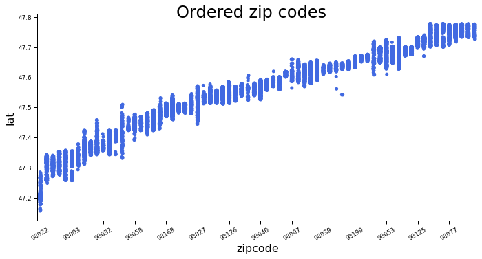
We can now see how the latitude can be nicely estimated from the zip codes (low spread of latitude within a zip code), but for each given latitude there are often at least five different zip codes. We have now seen how PPS can handle categorical features and asymmetric correlations and enable us to learn more about the correlations in our data.
In case you were not convinced by the above example, the less interesting example below shows more clearly how PPS is useful on complex correlations.
func = pd.DataFrame([[i, i**4-i**2+1] for i in np.linspace(-1, 1, 100)], columns=['x','y'])

#pcc = func.corr()
#print(ppscore.matrix(func).pivot('y','x','ppscore'))

ax = sns.scatterplot(data=func, x='x', y='y')
ax.set_title('PCC: 0.00 - PPS x->y: 0.86 - PPS y->x: 0.00')

From the figure we can clearly see how x can very easily estimate y (matching a PPS of 0.86), but y cannot estimate x (a PPS of 0). Likewise, as this is a non-linear correlation the PCC is 0. This nicely illustrates the usefulness of PPS to tells us whether x and y are asymmetrically correlated.
- PPS package: https://github.com/8080labs/ppscore
- Data used: https://www.kaggle.com/harlfoxem/house-price-prediction-part-1/data?select=kc_house_data.csv