
For the past couple of years I’ve been involved in running the Oxford University Scientific Society. We host weekly talks in Oxford during the Undergraduate Term, inviting speakers from all scientific disciplines to come and discuss their field with our members. Here are four important lessons I’ve learned from being involved!
Category Archives: Talks
A collection of prion factoids
It’s been several years since I last presented a talk on prions to OPIG, so I thought a neat way of getting up to date would be to read “The prion 2018 round tables“. What’s the current understanding and are we any closer to determining a structure of PrPSc?
Continue readingWhen OPIGlets leave the office
Hi everyone,
My blogpost this time around is a list of conferences popular with OPIGlets. You are highly likely to see at least one of us attending or presenting at these meetings! I’ve tried to make it as exhaustive as possible (with thanks to Fergus Imrie!), listing conferences in upcoming chronological order.
(Most descriptions are slightly modified snippets taken from the official websites.)
Making the most of your CPUs when using python
Over the last decade, single-threaded CPU performance has begun to plateau, whilst the number of logical cores has been increasing exponentially.
Like it or loathe it, for the last few years, python has featured as one of the top ten most popular languages [tiobe / PYPL]. That being said however, python has an issue which makes life harder for the user wanting to take advantage of this parallelism windfall. That issue is called the GIL (Global Interpreter Lock). The GIL can be thought of as the conch shell from Lord of the Flies. You have to hold the conch (GIL) for your thread to be computed. With only one conch, no matter how beautifully written and multithreaded your code, there will still only be one thread will be executed at any point in time.
So, you are interested in compound selectivity and machine learning papers?
At the last OPIG meeting, I gave a talk about compound selectivity and machine learning approaching to predict whether a compound might be selective. As promised, I hereby provide a list publications I would hand to a beginner in the field of compound selectivity and machine learning. Continue reading
ISMB 2018: Collaborative Structural Biology using Machine Learning and Jupyter Notebook
This post is a summary of the talk, Collaborative Structural Biology using Machine Learning and Jupyter Notebook, given by Fergus Imrie and Fergus Boyles at ISMB 2018. Materials for the experiments can be found here and here.
Myself and four other members of the Oxford Protein Informatics Group (a.k.a. OPIGlets) recently had the pleasure of attending the Intelligent Systems for Molecular Biology (ISMB) conference in Chicago. Organised by the International Society of Computational Biology (ISCB), ISMB is the largest computational biology conference in the world, with several thousand attendees.
Spread over four action-packed days in July (not including workshops/tutorial sessions), it was an eye-opening experience, showcasing the depth and breadth of computational biology research; particularly striking was the range of problems tackled, techniques applied, and data sources used.
I was fortunate enough to have the opportunity to present alongside my colleague, Fergus Boyles, as part of the 3DSIG Community of Special Interest (COSI). We led the first hands-on practical demonstration at 3DSIG, entitled “Collaborative Structural Biology using Machine Learning and Jupyter Notebook”. While a new format at the conference, with our presentation somewhat of an experiment, I understand the organising committee is keen to repeat the format next year.
In what follows, I’ll briefly outline the key themes and outcomes from our presentation. Full materials to reproduce all results presented in full can be found here and here.
Reproducibility crisis?
In a survey of 1,500 scientists by Nature in 2016 (link), more than 70% of participants had tried and failed to reproduce another scientist’s experiments, while 90% said there was a reproducibility crisis to some extent. Most striking, perhaps, was the revelation that “more than half have failed to reproduce their own experiments”!

Nature, 2016, M. Baker, 1,500 scientists lift the lid on reproducibility
While the focus of the survey was, admittedly, on traditional, lab-based, experimental research, this is certainly also an issue in computational approaches, with the machine learning community under the heaviest scrutiny.
This is clearly unsustainable and many efforts are being taken to address this across the scientific world. As one example, Nature has introduced a code and submission checklist that requires authors to submit custom algorithms or software that are central to the paper for peer review and editorial assessment. While only directly affecting a small portion of research, this is a big step in the right direction and I think we’re only going to see more of this in the future.
Software to the rescue?
With the rise of cloud computing, the open-source community, and much more, there is a plethora of software available that can be used to improve the accessibility of methods and improve the reproducibility of computational experiments. Below, I touch on a couple of general areas that are increasing used in computational pipelines and setups.
- Cloud computing (such as Amazon Web Services, Google Cloud, and Microsoft Azure) provides widely accessible, standardised compute environments, and allows the use of anything from a single core to near-HPC-level resources for a short period of time at relative inexpensive.
- Container solutions (such as Docker and Kubernets) allow developers to package an application, with all required libraries and dependencies, into a single executable for the end user, with no further dependencies.
Our approach
We didn’t use any of the above tools for purposes of our talk, but instead constructed our pipeline based on three other widely-used solutions: Conda, Project Jupyter, and Git/GitHub. For those unfamiliar, here is a brief overview of each.

- Conda is an open-source package and environment management system. It works by creating distinct virtual environments and installing standalone interpreters or compilers within that virtual environment. You can then install additional packages within that virtual environment, that are completely isolated and separate from your system default packages, and other virtual environments.

- For those of you who are familiar with the iPython notebook, Jupyter is an extension of this format to multiple languages. Jupyter provides an interactive browser-based coding environment in the form of a notebook, that can be thought of as similar to a lightweight IDE. The power of Jupyter notebooks comes from a combination of (1) the ability to intersperse code with markdown, which is much more human readable and friendly on the eye compared to traditional comments; (2) the cell-based format, where small pieces of code are contained in cells that can be run, and re-run, individually and without re-running the remainder of your code; (3) the ability to display inline figures, tables (among other things), rendering in HTML.
![]()
- Git is an open-source version control system. Version control is an essential bedrock of good programming that we don’t have time to go into in more detail, but long-story short, Git takes any headache out of version control.

- GitHub is a code hosting platform built for collaboration with Git at its core. Beyond a simple code repository, GitHub allows collaboration and development through two key features. “Forking” allows you to clone other projects, and either develop them yourself, or keep a record of a fixed version for integration within another project. “Pull requests” make large scale community collaboration projects possible, with users providing code for specific modifications for the original projects, which the owners/admin of the original project can choose to merge or reject.
Experiments
As a toy problem to showcase this approach to building a reproducible pipeline, we address the problem of protein classification according to the SCOP classification scheme. While the dataset we have shared contains examples of protein pairs that are in the same fold, superfamily, and family (as well as none of these), we focussed on the most straightforward task of determining whether a pair of proteins belong to the same family or not.

Our dataset is based on the Astral data set (06.02.2016 build), and consists of 8 pairwise features computed from the sequences of the two proteins. We won’t go into the details of the exact features here.
Using a simple random forest on these 8 pairwise features between the target and template protein, we achieved an accuracy of 88.0%, and an area under the receiver operative curve of 0.95. A confusion matrix and ROC curve summarising our results can be found below.

Instructions to reproduce these results, together with all materials needed, can be found here and here.
Conclusions
Reproducibility in science is facing a challenging time. All stakeholders, from researchers to funders and publishers, are placing more emphasis on work being reproducible, and are taking measures to ensure this. In computational research, in particular stochastic algorithms such as those prevalent throughout machine learning, the problem is no less serious, and on the face of it should be readily solvable.
In our demonstration, we have illustrated one approach to tackling this in a simple, efficient way. In addition, we only looked to tackle one possible problem or question, and only used a subset of the overall dataset. Please feel free to explore the dataset and pose your own questions. We’d love to hear from you if you do!
Acknowledgements
I’d like to thank all of OPIG for providing feedback on an early version of the talk. Crucially, I’d like to thank Dr Saulo de Oliveira who provided us with the dataset used in our exploratory analysis. Finally, I’d like to thank my co-presenter Fergus Bolyes, without whom I couldn’t have done this.
ISMB 2018 (Chicago): Summary of Interesting Talks/Posters
Catherine’s Selection
Network approach integrates 3D structural and sequence data to improve protein structural comparison
Why: Current graph mapping in protein structural comparison ignores sequence order of residues. Residues distant in sequence but close in 3D space are more important.
How: Introduce sequence order of residues, set a sequence-distance cutoff to consider structurally important residues, count the graphlet frequency and embed into PCA space.
Results: the new method is predictive of SCOP and CATH ‘groups’. Certain graphlets are enriched in alpha and beta folds.
Link: https://www.nature.com/articles/s41598-017-14411-y
Investigating the molecular determinants of Ebola virus pathogenicity
Why: Reston virus is the only Ebola virus that is not pathogenic to human
What they do: multiple sequence alignment to look for specificity determining positions (SDPs) using s3det, then predict the effect of each individual SDP on the stability of the protein with mCSM.
Results: VP40 SDPs alter octamer formation, structure hydrophobic core. VP24 SDPs leads to impair binding to KPNA5 in human, which inhibits interferon signalling.
Impact: only a few SDPs distinguish Reston VP24 from VP24 of others. Human-pathogenic Reston viruses may emerge.
Link: https://www.ncbi.nlm.nih.gov/pmc/articles/PMC5558184/#__ffn_sectitle
Computational Analysis Highlights Key Molecular Interactions and Conformational Flexibility of a New Epitope on the Malaria Circumsporozoite Protein and Paves the Way for Vaccine Design
Why: An antibody with a strong binding affinity was found in a group of subjects. This antibody prevents cleavage of the surface protein.
What they do: They found the linear epitope, crystallise the strong and medium binders and run a molecular dynamic simulation to find out the flexibility of the structures.
Results: The strong binder is less flexible. Moreover, the strong binder is similar to the germline sequence which may mean that this antibody could have been readily formed.
Link: https://www.nature.com/articles/nm.4512
—
Matt’s Selection
“Analysis of sequence and structure data to understand nanobody architectures and antigen interactions”
Laura S. Mitchell (Colwell Group)
University of Cambridge, UK
This poster detailed the work from Laura’s two most recent publications, which can be found here: https://doi.org/10.1002/prot.25497, https://doi.org/10.1093/protein/gzy017
They describe a comprehensive analysis of the binding properties of the 156 non-redundant nanobody-antigen (Nb-Ag) complexes in the PDB/SAbDab (October 2017). Their analyses include Nb sequence variability (both global and across the binding regions), contact maps of nanobody-antigen interactions by region, and the typical chemical properties of each paratope. Nb-Ag complexes are compared to a reference set of monoclonal antibody-antigen (mAb-Ag) complexes. This work is a key first step in advancing our understanding of Nb paratopes, and will aid the development of new diagnostics and therapeutics.
“OSPREY 3.0: Open-Source Protein Redesign for You, with Powerful New Features”
Jeffrey W. Martin (Donald Group)
Duke University, USA
OSPREY 3.0 (https://www.biorxiv.org/content/early/2018/04/23/306324) represents a large advance towards time-efficient continuous flexibility modelling of protein-protein interfaces.
Its new algorithms LUTE and BBK* allow for continuous rotamer flexibility searching and entropy-aware binding constant approximation in a much more efficient manner. The CATS algorithm also introduces local backbone flexibility as a long-awaited feature. This software now has a easy-to-use Python interface, and is fully Open-Source, making it an extremely attractive alternative to other proprietary protein design tools.
“Functional annotation of chemical libraries across diverse biological processes”
Scott Simpkins
University of Minnesota-Twin Cities, USA
This interesting talk detailed the work published in Nature Chemical Biology in September 2017 (https://doi.org/10.1038/nchembio.2436).
310 yeast gene-deletion mutants were isolated to perform chemical-genetic profile studies across six diverse small molecule high-throughput screening libraries. By studying which gene-deletion mutants were hypersensitive or resistant to each compound, the researchers could assign most members of each chemical library a probable functional annotation. Mapping back to gene-interaction profile data also allowed them to infer likely targets for some compounds. The GO annotations associated with these genes could then be used assess whether a given starting library is likely to contain promising starting-points that affect a given biological function. For example, the authors highlighted a deficiency across all libraries against the cellular processes of cytokinesis and ribosome biogenesis. Conversely, they found a large enrichment across all libraries for compounds likely to affect glycosylation or cell wall biogenesis. Compounds that target transcription and chromatin organisation were found to be enriched in certain datasets, and depleted in others. This genre of profiling provides researchers a way of judging a priori whether a given screening library is likely to contain promising lead compounds, given the functional role of the target of interest.
Storing your stuff with clever filesystems: ZFS and tmpfs
The filesystem is a a critical component of just about any operating system, however it’s often overlooked. When setting up a new server, the default filesystem options are often ticked and never thought about again. However, there exist a couple of filesystems which can provide some extraordinary features and speed. I’m talking about ZFS and tmpfs.
ZFS was originally developed by Oracle for their Solaris operating system, but has now been open-sourced and is freely available on linux. Tmpfs is a temporary file system which uses system memory to provide fast temporary storage for files. Together, they can provide outstanding reliability and speed for not very much effort.
Hard disk capacity has increased exponentially over the last 50 years. In the 1960s, you could rent a 5MB hard disk from IBM for the equivalent of $130,000 per month. Today you can buy for less than $600 a 12TB disk – a 2,400,000 times increase.

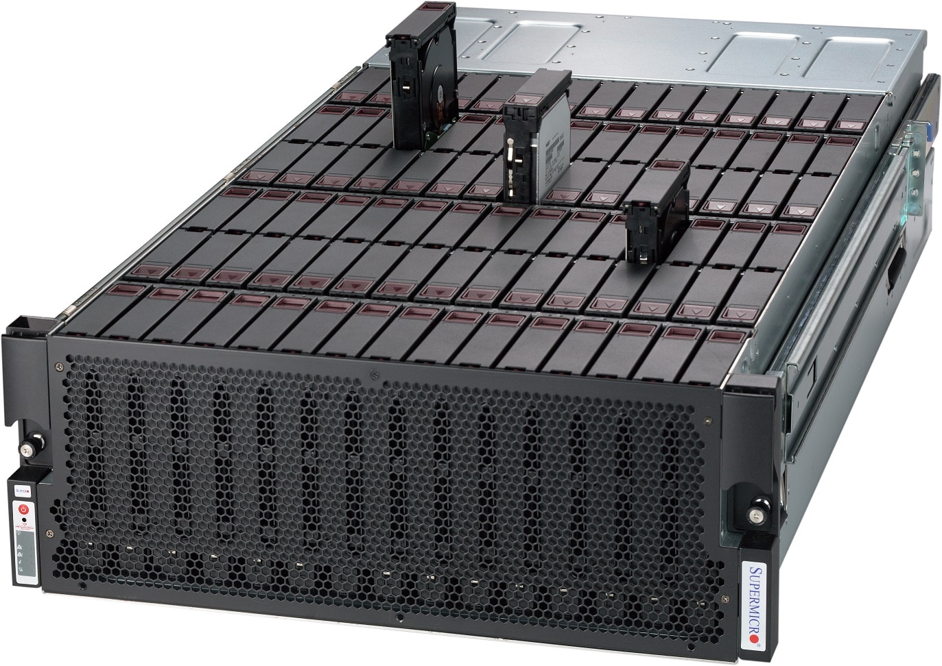
As storage technology has moved on, the filesystems which sit on top of them ideally need to be able to access the full capacity of those ever increasing disks. Many relatively new, or at least in-use, filesystems have serious limitations. Akin to “640K ought to be enough for anybody”, the likes of the FAT32 filesystem supports files which are at most 4GB on a chunk of disk (a partition) which can be at most 16TB. Bear in mind that arrays of disks can provide a working capacity of many times that of a single disk. You can buy the likes of a supermicro sc946ed shelf which will add 90 disks to your server. In an ideal world, as you buy bigger disks you should be able to pile them into your computer and tell your existing filesystem to make use of them, your filesystem should grow and you won’t have to remember a different drive letter or path depending on the hardware you’re using.
ZFS is a 128-bit file system, which means a single installation maxes out at 256 quadrillion zettabytes. All metadata is allocated dynamically so there isn’t the need to pre-allocate inodes and directories can have up to 2^48 (256 trillion) entries. ZFS provides the concept of “vdevs” (virtual devices) which can be a single disk or redundant/striped collections of multiple disks. These can be dynamically added to a pool of vdevs of the same type and your storage will grow onto the fresh hardware.
A further consideration is that both disks of the “spinning rust” variety and SSDs are subject to silent data corruption, i.e. “bit rot”. This can be caused by a number of factors even including cosmic rays, but the consequence is read errors when it comes time to retrieve your data. Manufacturers are aware of this and buried in the small print for your hard disk will be values for “unrecoverable read errors” i.e. data loss. ZFS works around this by providing several mechanisms:
- Checksums for each block of data written.
- Checksums for each pointer to data.
- Scrub – Automatically validates checksums when the system is idle.
- Multiple copies – Even if you have a single disk, it’s possible to provide redundancy by setting a copies=n variable during filesystem creation.
- Self-healing – When a bad data block is detected, ZFS fetches the correct data from a redundant copy and replaces it with the correct data.
An additional bonus to ZFS is its ability to de-duplicate data. Should you be working with a number of very similar files, on a normal filesystem, each file will take up space proportional to the amount of data that’s contained. As ZFS keeps checksums of each block of data, it’s able to determine if two blocks contain identical data. ZFS therefore provides the ability to have multiple pointers to the same file and only store the differences between them.
ZFS also provides the ability to take a point in time snapshot of the entire filesystem and roll it back to a previous time. If you’re a software developer, got a package that has 101 dependencies and you need to upgrade it? Afraid to upgrade it in case it breaks things horribly? Working on code and you want to roll back to a previous version? ZFS snapshots can be run with cron or manually and provide a version of the filesystem which can be used to extract previous versions of overwritten or deleted files or used to roll everything back to a point in time when it worked.

Similar to deduplication, a snapshot won’t take up any disk extra space until the data starts to change.
The other filesystem worth mentioning is tmpfs. Tmpfs takes part of the system memory and turns it into a usable filesystem. This is incredibly useful for systems which create huge numbers of temporary files and attempt to re-read them. Tmpfs is also just about as fast as a filesystem can be. Compared to a single SSD or a RAID array of six disks, tmpfs blows them out of the water speed wise.

Creating a tmpfs filesystem is simple:
First create your mountpoint for the disk:
mkdir /mnt/ramdisk
Then mount it. The options are saying make it 1GB in size, it’s of type tmpfs and to mount it at the previously created mount point:
mount –t tmpfs -o size=1024m tmpfs /mnt/ramdisk
At this point, you can use it like any other filesystem:
df -h
Filesystem Size Used Avail Use% Mounted on
/dev/sda1  218G 128G   80G  62% /
/dev/sdb1  6.3T 2.4T  3.6T  40% /spinnyrust
tank       946G 3.5G  942G   1% /tank
tmpfs      1.0G 391M  634M  39% /mnt/ramdisk
Slowing the progress of prion diseases
At present, the jury is still out on how prion diseases affect the body let alone how to cure them. We don’t know if amyloid plaques cause neurodegeneration or if they’re the result of it. Due to highly variable glycophosphatidylinositol (GPI) anchors, we don’t know the structure of prions. Due to their incredible resistance to proteolysis, we don’t know a simple way to destroy prions even using in an autoclave. The current recommendation[0] by the World Health Organisation includes the not so subtle: “Immerse in a pan containing 1N sodium hydroxide and heat in a gravity displacement autoclave at 121°C”.
There are several species including Water Buffalo, Horses and Dogs which are immune to prion diseases. Until relatively recently it was thought that rabbits were immune too. “Despite rabbits no longer being able to be classified as resistant to TSEs, an outbreak of ‘mad rabbit disease’ is unlikely”.[1] That being said, other than the addition of some salt bridges and additional H-bonds, we don’t know if that’s why some animals are immune.
We do know at least two species of lichen (P. sulcata and L. plumonaria) have not only discovered a way to naturally break down prions, but they’ve evolved two completely independent pathways to do so. How they accomplish this? We’re still not sure in fact, it was only last year that it was discovered that lichens may be composed of three symbiotic partnerships and not two as previously thought.[3]
With all this uncertainty, one thing is known: PrPSc, the pathogenic form of the Prion converts PrPC, the cellular form. Just preventing the production of PrPC may not be a good idea, mainly because we don’t know what it’s there for in the first place. Previous studies using PrP-knockout have shown hints that:
- Hematopoietic stem cells express PrP on their cell membrane. PrP-null stem cells exhibit increased sensitivity to cell depletion. [4]
- In mice, cleavage of PrP proteins in peripheral nerves causes the activation of myelin repair in Schwann Cells. Lack of PrP proteins caused demyelination in those cells. [5]
- Mice lacking genes for PrP show altered long-term potentiation in the hippocampus. [6]
- Prions have been indicated to play an important role in cell-cell adhesion and intracellular signalling.[7]
However, an alternative approach which bypasses most of the unknowns above is if it were possible to make off with the substrate which PrPSc uses, the progress of the disease might be slowed. A study by R Diaz-Espinoza et al. was able to show that by infecting animals with a self-replicating non-pathogenic prion disease it was possible to slow the fatal 263K scrapie agent. From their paper [8], “results show that a prophylactic inoculation of prion-infected animals with an anti-prion delays the onset of the disease and in some animals completely prevents the development of clinical symptoms and brain damage.”
[0] https://www.cdc.gov/prions/cjd/infection-control.html
[1] https://www.ncbi.nlm.nih.gov/pmc/articles/PMC3323982/
[2] https://blogs.scientificamerican.com/artful-amoeba/httpblogsscientificamericancomartful-amoeba20110725lichens-vs-the-almighty-prion/
[3] http://science.sciencemag.org/content/353/6298/488
[4] “Prion protein is expressed on long-term repopulating hematopoietic stem cells and is important for their self-renewal”. PNAS. 103 (7): 2184–9. doi:10.1073/pnas.0510577103
[5] Abbott A (2010-01-24). “Healthy prions protect nerves”. Nature. doi:10.1038/news.2010.29
[6] Maglio LE, Perez MF, Martins VR, Brentani RR, Ramirez OA (Nov 2004). “Hippocampal synaptic plasticity in mice devoid of cellular prion protein”. Brain Research. Molecular Brain Research. 131 (1-2): 58–64. doi:10.1016/j.molbrainres.2004.08.004
[7] Málaga-Trillo E, Solis GP, et al. (Mar 2009). Weissmann C, ed. “Regulation of embryonic cell adhesion by the prion protein”. PLoS Biology. 7 (3): e55. doi:10.1371/journal.pbio.1000055
[8] http://www.nature.com/mp/journal/vaop/ncurrent/full/mp201784a.html
Strachey Lecture – “Artificial Intelligence and the Future” by Dr. Demis Hassabis
For this week’s group meeting, some of us had the pleasure of attending a very interesting lecture by Dr. Demis Hassabis, founder of Deep Mind. Personally, I found the lecture quite thought-evoking and left the venue with a plethora of ideas sizzling in my brain. Since one of the best ways to end mental sizzlingness is by writing things down, I volunteered to write this week’s blog post in order to say my peace about yesterday’s Strachey Lecture.
Dr. Hassabis began by listing some very audacious goals: “To solve intelligence” and “To use it to make a better world”. At the end of his talk, someone in the audience asked him if he thought it was possible to achieve these goals (“to fully replicate the brain”), to which he responded with a simple there is nothing that tells us that we can’t.
After his bold introductory statement, Dr. Hassabis pressed on. For the first part of his lecture, he engaged the audience with videos and concepts of a reinforcement learning agent trained to learn and play several ATARI games. I was particularly impressed with the notion that the same agent could be used to achieve a professional level of gaming for 49 different games. Some of the videos are quite impressive and can be seen here or here. Suffice to say that their algorithm was much better at playing ATARi than I’ll ever be. It was also rather impressive to know that all the algorithm received as input was the game’s score and the pixels on the screen.
Dr. Hassabis mentioned in his lecture that games provide the ideal training ground for any form of AI. He presented several reasons for this, but the one that stuck with me was the notion that games quite often present a very simplistic and clear score. Your goal in a game is usually very well defined. You help the frog cross the road or you defeat some aliens for points. However, what I perceive to be the greatest challenge for AI is the fact that real world problems do not come with such a clear-cut, incremental score.
For instance, let us relate back to my particular scientific question: protein structure prediction. It has been suggested that much simpler algorithms such as Simulated Annealing are able to model protein structures as long as we have a perfect scoring system [Yang and Zhou, 2015]. The issue is, currently, the only way we have to define a perfect score is to use the very structure we are trying to predict (which kinda takes the whole prediction part out of the story).
Real world problems are hard. I am sure this is no news to anyone, including the scientists at Deep Mind.
During the second part of his talk, Dr. Hassabis focused on AlphaGo. AlphaGo is Deep Mind’s effort at mastering the ancient game of Go. What appealed to me in this part of the talk is the fact that Go has such a large number of possible configurations that devising an incremental score is no simple task (sounds familiar?). Yet, somehow, Deep Mind scientists were able to train their algorithm to a point where it defeated a professional Go player.
Their next challenge? In two weeks, AlphaGo will face the professional Go player with the highest number of titles in the last decade (the best player in the world?). This makes me reminiscent of when Garry Kasparov faced Deep Blue. After the talk, my fellow OPIG colleagues also seemed to be pretty excited about the outcome of the match (man vs. food computer).
Dr. Hassabis finished by saying that his career goal would be to develop AI that is capable of helping scientists tackle the big problems. From what I gather (and from my extremely biased point of view; protein structure prediction mindset), AI will only be able to achieve this goal once it is capable of coming up with its own scores for the games we present it to play with (hence developing some form of impetus). Regardless of how far we are from achieving this, at least we have a reason to cheer for AlphaGo in a couple of weeks (because hey, if you are trying to make our lives easier with clever AI, I am all up for it).