Category Archives: Group Meetings

What we discuss during cake at our Tuesday afternoon group meetings

Viewing ligands in twilight electron density

In this week’s journal club we discussed an excellent review paper by E. Pozharski, C. X. Weichenberger and B. Rupp investigating crystallographic approaches to protein-ligand complex elucidation. The paper assessed and highlighted the shortcomings of deposited PDB structures containing ligand-protein complexes. It then made suggestions for the community as a whole and for researchers making use of ligand-protein complexes in their work.

The paper discussed:

The difficulties in protein ligand complex elucidation
The tools to assess the quality of protein-ligand structures both qualitative and quantitative
The methods used describing their analysis of certain PDB structures
Some case studies visually demonstrating these issues
Some practical conclusions for the crystallographic community
Some practical conclusions for non-crystallographer users of protein-ligand complex structures from the PDB

The basic difficulties of ligand-protein complex elucidation

Ligands have less than 100% occupancy – sometimes significantly less and thus will inherently show up less clearly in the overall electron density.
Ligands make small contributions to the overall structure and thus global quality measures , such as r-factors, will be affected only minutely by the ligand portion of the structure being wrong
The original basis model needs to be used appropriately. The r-free data from the original APO model should be used to avoid model bias

The following are the tools available to inspect the quality of agreement between protein structures and their associated data.

Visual inspection of the Fo-Fc and 2Fo-Fc maps,using software such as COOT, is essential to assess qualitatively whether a structure is justified by the evidence.
Use of local measures of quality for example real space correlation coefficients (RSCC)
Their own tool, making use of the above as well as global quality measure resolution

Methods and results

In a separate publication they had analysed the entirety of the PDB containing both ligands and published structure factors. In this sample they demonstrate 7.6% had RSCC values of less than 0.6 the arbitrary cut off they use to determine whether the experimental evidence supports the model coordinates.

Figure to show an incorrectly oriented ligand (a) and its correction (b)

An incorrectly oriented ligand (a) and its correction (b). In all of these figures Blue is the 2mF_oDF_c map contoured at 1σ and Green and Red are positive and negative conturing of the mF_oDF_c map at 3σ

In this publication they visually inspected a subset of structures to assess in more detail how effective that arbitrary cutoff is and ascertain the reason for poor correlation. They showed the following:

(i) Ligands incorrectly identiﬁed as questionable,false positives(7.4%)
(ii) Incorrectly modelled ligands (5.2%)
(iii) Ligands with partially missing density (29.2%).
(iv) Glycosylation sites (31.3%)
(v) Ligands placed into electron density that is likely to
originate from mother-liquor components
(vi) Incorrect ligand (4.7%)
(vii) Ligands that are entirely unjustiﬁed by the electron
density (11.9%).

The first point on the above data is that the false-positive rate using RSCC of 0.6 is 7.4%. This demonstrates that this value is not sufficient to accurately determine incorrect ligand coordinates. Within the other categories all errors can be attributed to one of or a combination of the following two factors:

The inexperience of the crystallographer being unable to understand the data in front of them
The wilful denial of the data in front of the crystallographer in order that they present the data they wanted to see

Figure to show a ligand placed in density for a sulphate ion from the mother liquor (a) and it's correction (b)

A ligand incorrectly placed in density for a sulphate ion from the mother liquor (a) and it’s correction (b)

The paper observed that a disproportionate amount of poor answers was derived from glycosylation sites. In some instances these observations were used to inform the biochemistry of the protein in question. Interestingly this follows observations from almost a decade ago, however many of the examples in the Twilight paper were taken from 2008 or later. This indicates the community as a whole is not reacting to this problem and needs further prodding.

Figure to show an incomplete glycosylation site inaccurately modeled

Conclusions and suggestions

For inexperienced users looking at ligand-protein complexes from the PDB:

Inspect the electron density map using COOT if is available to determine qualitatively is their evidence for the ligand being there
If using large numbers of ligand-protein complexes, use a script such as Twilight to find the RSCC value for the ligand to give some confidence a ligand is actually present as stated

For the crystallographic community:

Improved training of crystallographers to ensure errors due to genuine misinterpretation of the underlying data are minimised
More submission of electron-density maps, even if not publically available they should form part of initial structure validation
Software is easy to use but difficult to analyse the output

GPGPUs for bioinformatics

As the clock speed in computer Central Processing Units (CPUs) began to plateau, their data and task parallelism was expanded to compensate. These days (2013) it is not uncommon to find upwards of a dozen processing cores on a single CPU and each core capable of performing 8 calculations as a single operation. Graphics Processing Units were originally intended to assist CPUs by providing hardware optimised to speed up rendering highly parallel graphical data into a frame buffer. As graphical models became more complex, it became difficult to provide a single piece of hardware which implemented an optimised design for every model and every calculation the end user may desire. Instead, GPU designs evolved to be more readily programmable and exhibit greater parallelism. Top-end GPUs are now equipped with over 2,500 simple cores and have their own CUDA or OpenCL programming languages. This new found programmability allowed users the freedom to take non-graphics tasks which would otherwise have saturated a CPU for days and to run them on the highly parallel hardware of the GPU. This technique proved so effective for certain tasks that GPU manufacturers have since begun to tweak their architectures to be suitable not just for graphics processing but also for more general purpose tasks, thus beginning the evolution General Purpose Graphics Processing Unit (GPGPU).

Improvements in data capture and model generation have caused an explosion in the amount of bioinformatic data which is now available. Data which is increasing in volume faster than CPUs are increasing in either speed or parallelism. An example of this can be found here, which displays a graph of the number of proteins stored in the Protein Data Bank per year. To process this vast volume of data, many of the common tools for structure prediction, sequence analysis, molecular dynamics and so forth have now been ported to the GPGPU. The following tools are now GPGPU enabled and offer significant speed-up compared to their CPU-based counterparts:

Application	Description	Expected Speed Up	Multi-GPU Support
Abalone	Models molecular dynamics of biopolymers for simulations of proteins, DNA and ligands	4-29x	No
ACEMD	GPU simulation of molecular mechanics force fields, implicit and explicit solvent	160 ns/day GPU version only	Yes
AMBER	Suite of programs to simulate molecular dynamics on biomolecule	89.44 ns/day JAC NVE	Yes
BarraCUDA	Sequence mapping software	6-10x	Yes
CUDASW++	Open source software for Smith-Waterman protein database searches on GPUs	10-50x	Yes
CUDA-BLASTP	Accelerates NCBI BLAST for scanning protein sequence databases	10	Yes
CUSHAW	Parallelized short read aligner	10x	Yes
DL-POLY	Simulate macromolecules, polymers, ionic systems, etc on a distributed memory parallel computer	4x	Yes
GPU-BLAST	Local search with fast k-tuple heuristic	3-4x	No
GROMACS	Simulation of biochemical molecules with complicated bond interactions	165 ns/Day DHFR	No
GPU-HMMER	Parallelized local and global search with profile Hidden Markov models	60-100x	Yes
HOOMD-Blue	Particle dynamics package written from the ground up for GPUs	2x	Yes
LAMMPS	Classical molecular dynamics package	3-18x	Yes
mCUDA-MEME	Ultrafast scalable motif discovery algorithm based on MEME	4-10x	Yes
MUMmerGPU	An open-source high-throughput parallel pairwise local sequence alignment program	13x	No
NAMD	Designed for high-performance simulation of large molecular systems	6.44 ns/days STMV 585x 2050s	Yes
OpenMM	Library and application for molecular dynamics for HPC with GPUs	Implicit: 127-213 ns/day; Explicit: 18-55 ns/day DHFR	Yes
SeqNFind	A commercial GPU Accelerated Sequence Analysis Toolset	400x	Yes
TeraChem	A general purpose quantum chemistry package	7-50x	Yes
UGENE	Opensource Smith-Waterman for SSE/CUDA, Suffix array based repeats finder and dotplot	6-8x	Yes
WideLM	Fits numerous linear models to a fixed design and response	150x	Yes

It is important to note however, that due to how GPGPUs handle floating point arithmetic compared to CPUs, results can and will differ between architectures, making a direct comparison impossible. Instead, interval arithmetic may be useful to sanity-check the results generated on the GPU are consistent with those from a CPU based system.

PredyFlexy – Predicting Protein Flexibility

An example output of PredyFlexy

My presentation focused on a method to predict protein flexibility – PredyFlexy. There is a webserver, and it is described in their paper (de Brevern et. al 2012). The method is covered much more explicitly in the paper Predicting protein flexibility through the prediction of local structures (Bornot et al. 2011). This work builds on earlier papers (which are mentioned on the front page of the webserver, some of which I will mention later). In terms of people, Alexandre G. de Brevern, Aurelie Bornot, and Catherine Etchebest are authors common to all of these papers.

The concept is simple; there is a library of ‘Local Structure Prototypes’ or LSPs. These LSPs are 11 residue fragments, and have structure and flexibility associated with them, which are derived from a set of protein structures and molecular dynamics simulations. Each LSP has a SVM (support vector machine) ‘expert’ to score how likely a given sequence profile is to have said structure. A 21 residue window is used to determine the LSP of the central 11 residues within this window.

So, the user inputs a sequence, which gets Psi-Blasted to give a sequence profile. The 5 most probable LSPs for each atom are determined using the SVM experts. Then the predicted flexibility of each atom is given by the average flexibility of these 5 LSPs. There is a confidence index to the predictions, which comes from assessing the discriminative power of the SVMs. Regions predicted to have LSP with more accurate SVMs will have a high confidence index.

Examples of Local Structure Prototypes. Taken from the supplementary information of ‘Predicting protein flexibility through the prediction of local structures’ – Aurélie Bornot, Catherine Etchebest, Alexandre G. de Brevern, Proteins 79, 3, 839–852, 2011

So, the concept seems simple, but you are probably wondering, what are these LSPs? To answer that, we have to delve into the literature. ‘Bayesian probabilistic approach for predicting backbone structures in terms of protein blocks‘, published in 2000, and with Alexandre G. de Brevern as first author, is the sensible place to start. This introduced the concept of protein blocks, which is in effect a structural alphabet. These are 5 residue fragments (described by 8 dihedral angles), and there are 16 of them (there are pretty pictures in the supplementary data 1 of this paper). Local structure prototypes are made up of these protein blocks, which were first used to predict structure, in a 2006 paper – Assessing a Novel Approach for Predicting Local 3D Protein Structures from Sequence (again, with the same authors). LSPs are 11 residue fragments, made from 7 overlapping protein blocks. Obviously there are lots of combinations to the protein blocks that can give 11 residue fragments. These combinations are clustered into 120 groups. Each group is represented by the fragment within the cluster that is closest to all other fragments within the cluster, based on C-alpha RMSD. Hence 120 LSPs.

The other pertinent question is, where does the flexibility data come from? Well, they did some MD simulations (see Bornot et al. 2011 for details) and took b-factors from the structures. They normalised these, by calculating the number of standard deviations away from the mean for each structure. Each LSP was attributed a b-factor and RMSF, which was the mean value for the central residue of every instance of the LSP in the data set. Additionally, each fragment in the data set was classed as ‘rigid’, ‘flexible’, or ‘intermediate’ based on its normalized RMSF and B-factor. Each LSP was given a probability of belonging to each of these classes based on the frequency of fragments that belonged to that LSP being in each class. The figure here (taken from Bornot et al. 2011) shows the interesting weak correlation between normalised B-factor and normalised RMSF.

Normalised B-factor values according to normalized RMSF values as determined from molecular dynamics simulations. From Bornot et al 2011. Blue points represent rigid fragments, red flexible ones, and green points intermediate fragments.

Bornot et al. 2011 also gives us a guide to the ability of this prediction method (see table II). In predicting the class of fragments (rigid, intermediate or flexible), it gets the correct class about half the time. For 40% of rigid and flexible cases, the class is predicted as ‘intermediate’. Prediction rate is also strongly correlated with flexibility – more flexible regions have much poorer prediction rates. Which is not great, as we already know that most alpha helices are rigid. However, the confidence index does give a good guide as to what to trust. I could speculate that might results in an output that tells us that helices and sheets are definitely rigid, and other elements are possibly flexible. Which would not be particularly useful, but given there are few comparable tools, something is better than nothing.

Protein flexibility is hard; experimentally determining it is difficult (and even MD simulations take a while), and people can argue about how relevant the experimental methods are (and we frequently do in our group meetings). So, like most predictive methods, a relatively fast (and simple) way to get some information about your problem is always going to be useful. If only to guide you to where you might focus your attention.

Journal club: Simultaneous Femtosecond X-ray Spectroscopy and Diffraction of Photosystem II at Room Temperature

In the last journal club we covered the paper Simultaneous Femtosecond X-ray Spectroscopy and Diffraction of Photosystem II at Room Temperature (Kern et al., 2013), currently still in Science Express.

Structure of Photosystem II, PDB 2AXT
CC BY-SA 3.0 Curtis Neveu

This paper describes an experiment on the Photosystem II (PSII) protein complex. PSII is a large protein complex consisting of about 20 subunits with a combined weight of ca. 350 kDa. As its name suggests, this complex plays a crucial role in photosynthesis: it is responsible for the oxidation (“splitting up”) of water.

In the actual experiment (see the top right corner of Figure 1 in the paper) three experimental methods are combined: PSII microcrystals (5-15µm) are injected from the top into the path of an X-ray pulse (blue). Simultaneously, an emission spectrum is recorded (yellow, detector at the bottom). And finally in a separate run the injected crystals are treated (‘pumped’) with a visible laser (red) before they hit the X-ray pulse.

Let’s take a look at each of those three in a little more detail.

X-ray diffraction (XRD)

In a standard macromolecular X-ray crystallography experiment a crystal containing identical molecules of interest (protein) at regular, ordered lattice points is exposed to an X-ray beam. Some X-rays are elastically scattered and cause a diffraction pattern to form on a detector. By analysing the diffraction patterns of a rotating crystal it is possible to calculate the electron density distribution of the molecule in question, and thus determine its three dimensional structure.

An intense X-ray beam however also systematically damages the sample (Garman, 2010). For experiments using in-house X-ray generators or synchrotrons it is therefore recommended not to exceed a total dose of 30 MGy on any one crystal (Owen et al., 2006).

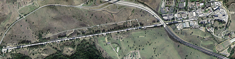
Aerial view of the LCLS site. The accelerator is 3.2 kilometres long.

The experiment described in the current paper however was not conducted using a run-of-the-mill synchrotron, but with the Linac Coherent Light Source (LCLS), an X-ray free electron laser. Here each diffraction image results from an individual crystal exposed to a single X-ray pulse of about 50 femtoseconds, resulting in a peak dose of ~150 MGy. Delivering these extreme doses in very short X-ray pulses lead to the destruction of the sample via a coulomb explosion.

As the sample is destroyed only one diffraction image can be taken per crystal. This causes two complications: Firstly, a large number of sample crystals are required. This explains why the experiment required a total beam time of 6 hours and involved over 2.5 million X-ray shots and processing an equal number of diffraction images. Secondly, the resulting set of (usable) diffraction images are an unordered, random sampling of the crystal orientation space. This presents a computational challenge unique to XFEL setups: before the diffraction data can be integrated, the orientation of the crystal lattice needs to be determined for each individual diffraction image.

X-ray diffraction allows us to obtain a electron density map of the entire unit cell, and therefore the entire crystal. But we can only see ordered areas of the crystal. To really see small molecules in solvent channels, or the conformations of side chains on the protein surface they need to occupy the same positions within each unit cell. For most small molecules this is not the case. This is why you will basically never see compounds like PEGs or Glycerol in your electron density maps, even though you used them during sample preparation. For heavy metal compounds this is especially annoying. They disproportionately increase the X-ray absorption (Holton, 2009; with a handy table 1) and therefore shorten the crystal’s lifetime. But they do not contribute to the diffraction pattern (And that is why you should back-soak; Garman & Murray, 2003).

X-ray emission spectroscopy (XES)

PSII contains a manganese cluster (Mn₄CaO₅). This cluster, as with all protein metallocentres, is known to be highly radiation sensitive (Yano et al., 2005). Apparently at a dose of about 0.75 MGy the cluster is reduced in 50% of the irradiated unit cells.

Diffraction patterns represent a space- and time-average of the electron density. It is very difficult to quantify the amount of reduction from the obtained diffraction patterns. There is however a better and more direct way of measuring the states of the metal atoms: X-ray emission spectroscopy.

Basically the very same events that cause radiation damage also cause X-ray emissions with very specific energies, characteristic for the involved atoms and their oxidation state. An Mn^IVO₂ energy spectrum looks markedly different to an Mn^IIO spectrum (bottom right corner of Figure 1).

The measurements of XRD and XES are taken simultaneously. But, differently to XRD, XES does not rely on crystalline order. It makes no difference whether the metallocentres move within the unit cell as a result of specific radiation damage. Even the destruction of the sample is not an issue: we can assume that XES will record the state of the clusters regardless of the state of the crystal lattice – up to the point where the whole sample blows up. But at that point we know that due to the loss of long-range order the X-ray diffraction pattern will no longer be affected.

The measurements of XES therefore give us a worst-case scenario of the state of the manganese cluster in the time-frame where we obtained the X-ray diffraction data.

Induced protein state transition with visible laser

Another neat technique used in this experiment is the activation of the protein by a visible laser in the flight path of the crystals as they approach the X-ray interaction zone. With a known crystal injection speed and a known distance between the visible laser and the X-ray pulse it becomes possible to observe time-dependent protein processes (top left corner of Figure 1).

What makes this paper special? (And why is it important to my work?)

It has been theorized and partially known that the collection of diffraction data using X-ray free electron lasers outruns traditional radiation damage processes. Yet there was no conclusive proof – up until now.

This paper has shown that the XES spectra of the highly sensitive metallocentres do not indicate any measurable (let alone significant) change from the idealized intact state (Figure 3). Apparently the highly sensitive metallocentres of the protein stay intact up to the point of complete sample destruction, and certainly well beyond the point of sample diffraction.

Or to put another way: even though the crystalline sample itself is destroyed under extreme conditions, the obtained diffraction pattern is – for all intents and purposes – that of an intact, pristine, zero dose state of the crystal.

This is an intriguing result for people interested in macromolecular crystallography radiation damage. In a regime of absurdly high doses, where the entire concept of a ‘dose’ for a crystal breaks down (again), we can obtain structural data with no specific radiation damage present at the metallocentres. As metallocentres are more susceptible to specific radiation damage it stands to reason that the diffraction data may be free of all specific damage artefacts.

It is thought that most deposited PDB protein structures containing metallocentres are in a reduced state. XFELs are being constructed all over the world and will be the next big thing in macromolecular crystallography. And now it seems that the future of metalloproteins got even brighter.

Journal Club: Can Linear Progamming (LP) be useful to us?

Linear programming (LP) is known as a fast and powerful computational technique. It has been applied to a large range of problems in finances and economics, but it is not very popular among us bioinformaticians, computational biologists, and the likes.

Linear Programming is all about find feasible solutions that satisfy a series of constraints (usually represented by inequalities). Does it sound like a familiar problem to bioinformaticians and computational biologists out there?

Source: http://hotmath.com/hotmath_help/topics/linear-programming.html

This leaves room for some questioning: can biological phenomena be modelled or simplified under the assumption of linearity? Furthermore, can LP be used to tackle the many difficult problems posed in our field? Perhaps an even bigger question: why would any of us use Linear Programming instead of another type of linear modelling? What are the advantages of it?

I will not incur in explaining the particulars of LP here. There is a plethora of materials available online (Wikipedia and Wolfram are accessible starting points) that detail Linear Programming. For those eager for something more substantial, V. Chvatal’s Linear Programming and Dantzig’s Linear Programming and Extensions are two good texts on the subject.

During this week’s journal club, I discussed an article that attempted to use Linear Programming to devise knowledge-based Docking Potentials (DP) tailored for transient protein-protein complexes. Transient complexes tend to be under-represented on the PDB, mostly due to the inherent difficulties of crystallizing such complexes. Hence, the development of knowledge-based potentials for these special cases of protein interaction is drastically hindered by a sample size limitation.

A cartoon representation of a transient complex between Azurin (cyan) and its partner Cytochrome C551 (dark blue) from Pseudomonas aeruginosa. Transient protein complexes are hard to crystallize, hence, under-represented on the PDB.

Source: Bizzarri AR, Brunori E, Bonanni B, Cannistraro S. Docking and molecular dynamics simulation of the Azurin–Cytochrome c551 electron transfer complex. J. Mol. Recognit. 2007; 20: 122–131

To offset such limitation, it would be ideal if one could extrapolate information from decoys (non-native conformations obtained from computational docking tools) in order to improve the Docking potentials. Furthermore, in an ideal world, one would also address the bias introduced by homology/sequence similarity between the existing proteins in the available structures of transient complexes.

The author of the article “Designing coarse grained-and atom based-potentials for protein-protein docking – Tobi D. – BMC Structural Biology 2010, 10:40 doi:10.1186/1472-6807-10-40 ” claims that LP can address such issues by incorporating information from the decoys as linear constraints to the model. The article describes a linear problem, in which the aim is to minimize the variance of how much the non-native energy potentials differ from the native ones. Also, they impose the constraints that native structures must have a lower energy than all of the non-native structures for a given complex (lower in this case is good).

The energy is defined as a weighted sum of the counts of specific interaction types on the complex interface. In their work, the author employed two models: an atom-based model and a side chain-based model. These models are used to classify atoms into groups and to simplify calculations. Initially, they define boolean (one-step) interactions: two atoms interact if they are within a cutoff distance of each other. This cutoff varies according to the type of atoms involved. The initial model led to a state of infeasibility, and it was then replaced by a two-step model, where you have strong and weak interactions and two sets of cutoff (this leads to twice as many unknowns in the LP model).

Well, does it work? How does it fair against other existing knowledge-based DPs?

Source: Designing coarse grained-and atom based-potentials for protein-protein docking. – Tobi D. – BMC Structural Biology 2010, 10:40 doi:10.1186/1472-6807-10-40

Despite the lack of brilliant results or any apparent improvement compared to the state-of-art, the potentials described in the article seem to slightly outperform ZDOCK2.3’s scoring functions.

This may actually speak in favour of the applicability of LP to problems in our area. In the case presented during the journal club, an LP approach produced comparable results to more conventional techniques.

Perhaps the best answer to “why should I use LP?” is that it is an unconventional, creative solution. It is significantly fast and, therefore, easy to try out depending on your problem. Science is all about experimentation, after all. Why would you not try a different technique if you have the means to?

The moral of the story: it is good to think outside the box, as long as you keep your feet on the ground.

Image Source: http://www.designthenewbusiness.com/blog/documenting/thinking-inside-the-box.html

Check the article discussed in the post here.

Journal Club: Protein structure model refinement using fragment-guided MD

For this week’s journal club I presented this paper by Jian et al from the Zhang Lab. The paper tackles the problem of refining protein structure models using molecular dynamics (MD).

The most successful protocols for building protein structure models have been template-based methods. These involve selecting whole or parts of known protein structures and assembling them to form an initial model of the target sequence of interest. This initial model can then be altered or refined to (hopefully) achieve higher accuracy. One method to make these adjustments is to use molecular dynamics simulations to sample different conformations of the structure. A “refined” model can then be taken as a low-energy state that the simulation converges to. However, whilst physics-based potentials are effective for certain aspects of refinement (e.g. relieving clashes between side chain atoms), the task of actually improving overall model quality has so far proved to be too ambitious.

The Method

In this paper entitled “Atomic-Level Protein Structure Refinement Using Fragment-Guided Molecular Dynamics Conformation Sampling,” Jian et al demonstrate that current MD refinement methods have little guarantee of making any improvement to the accuracy of the model. They therefore introduce a technique of supplementing physics-based potentials with knowledge about fragments of structures that are similar to the protein of interest.

The method works by using the initial model to search for similar structures within the PDB. These are found using two regimes. The first is to search for global templates by assessing the TMscore of structures to the whole initial model. The second is to search for fragments of structures by dividing the initial model into continuous 3 secondary structure elements. From these sets of templates and the initial model, the authors can generate a bespoke potential for the model based on the distances between Cα atoms. By doing this, additional information about the likely global topology of the protein can be incorporated into a molecular dynamics simulation. The authors claim that this enables the MD energy landscape is therefore reshaped from being “golf-course-like” being “funnel-like”. Essentially, the MD simulations are guided to sample conformations which are likely (as informed by the fragments) to be close to the target protein structure.

A schematic of the FG-MD refinement procedure

Does it work?

As a full solution to the problem of protein structure model refinement, the results are far from convincing. Quality measures show improvement in only the second or third decimal place from the initial model to the refined model. Also, as might be expected, the degree to which the model quality is improved is dependent on the accuracy of the initial of the model.

However, what is important about this paper is that, although small, the improvements made do exist in a systematic fashion. Previously, attempts to refine a model using MD not only failed to improve its accuracy but would be likely to reduce its quality. Fragment-guided MD (FG-MD) and the explicit inclusion of a hydrogen bonding potential, is not only able to improve the conformations of side chains but also improve (or at least not destroy) the global backbone topology of a model.

Dependence of the energy of a model on its TM-Score to the native structure. In black is the energy as measure using the AMBER99 energy function. In grey is the corresponding funnel-like shape of the FG-MD energy function.

This paper therefore lays the groundwork for the development of further refinement methods that incorporate the knowledge from protein structure fragments with atomically detailed energy functions. Given that the success of the method is related to the accuracy of the initial model, there may be scope for developing similar techniques to refine models of specific proteins where modelling quality is already good. e.g. antibodies.

Journal club: Improving the selectivity of antimicrobial peptides

Last wednesday I talked about this paper which is about antimicrobial peptides. First I should say even though many of the authors are French this particular group was unknown to me and it was only the subject tackled which caught my eye – no patriotism, as it should become obvious in the following paragraphs. More precisely, being a bit of an outlier in OPIG (as I spend all my time in the biochemistry building doing Molecular Dynamics (MD) simulations) I was curious to get feedback from OPIG members on the sequence processing method developed in this article.

So what are antimicrobial peptides (AMP) and what do we want to do with them?

These are peptides able to kill bacteria in a rather unspecific manner: instead of targeting a particular membrane receptor AMP appear to lyse bacterial membrane via poration mechanisms which are not totally understood but relies on electrostatic interactions and lead to cell leakage and death. This mode of action means it is difficult for bacteria to develop resistance (they can’t change their entire membrane) and AMP are extensively studied as promising antibiotics. However, the therapeutic potential of AMP is severely limited by the fact that they are also often toxic to eukaryotic cells – this is the downside of their rather unspecific membrane lytic activity.

If AMP are to become useful antibiotic it is therefore important to maximise their activity against bacterial cells while limiting it against eukaryotic cells. This is precisely the problem tackled by this paper.

The ratio between the desired and not desired activity of AMP can be measured by the therapeutic index (TI) which is defined in this paper as:

TI = HC50 / MIC

where HC50 is the AMP concentration needed to kill 50% of red blood cells and MIC is the minimal inhibitory concentration against bacteria. The higher the TI the better the AMP for therapeutic use and the authors presents a method to identify mutations (single or double) in order to increase the TI of a given sequence.

What did the authors do?

Their method relies on a new way to describe AMP properties, which the authors called the sequence moment and which was built to reflect the asymmetry along the peptide chain regarding the property of interest. The rationale underlying this is that there is a functional asymmetry in the peptide chain, with the N terminal region being “more important for activity and selectivity of AMPs” – this claim is based on a reference from 2000 in which it is shown that in the peptides studied mutations in the N-terminus region are more likely than that in the C-terminus region to result in a decrease in AMP activity.

The derivation of the sequence moment is interesting and illustrated in the figure below. The AMP sequence is projected on a 90 degrees arc, with the N terminus on the y axis. The metric of interest is then plotted for each residue as a vector (tiny arrows in the figure) with the same origin as the arc and the length and direction of which depends on the metric value and the orientation. The mean value of the metric for the AMP sequence is then obtained by summing the positional vectors together (big arrows).

With this method the authors are able to get a mean value for the metric of interest which also contains information on the distribution along the AMP sequence of the metric of interest.

Interestingly, the descriptor used by the authors is actually the angle difference between the arrows obtained when calculating the sequence moment using two different hydrophobicity scales (Janin’s and Guy’s) – see red and blue arrows in the figure above.

The authors claim that the cosine of this angle, termed descriptor D, correlates well with the TI of AMP according to the following linear relation:

TI = 50.1 – 44.8*D

Long story short the authors then describe how they implemented a software, called Mutator and available here, which takes a sequence as input and based on a set of 26 best AMP (defined as having a TI > 20 and less than 70% sequence homology between them) suggest single or double mutations to improve its TI based on the method and relationship above. They then test their predictions experimentally for 2 peptides (Ascaphin-8 and XT-7) and it appears that the analogues suggested by the Mutator do have a much higher TI than their parent sequence.

What do we think about it?

Although this paper presents a method which seemingly gives impressive results I have 2 major problems with it.

The first one would be that the D descriptor has no rationale nor clear signification which makes interpreting the results difficult. Which sequence property does this descriptor capture? At best it can be said that when D is small the two hydrophobicity scales differ widely for the sequence studied (arrows at a 90 degrees angle), whereas they agree when D is close to 1. It would then be necessary to go back to how the scales were derived to understand what is being picked-up here, if anything.

Second, there is no proper statistical analysis of the significance of the results obtained. As noted by OPIG members the peptides studied are all fairly similar,and the less than 70% pairwise identity rule used for the training does not guarantee much diversity. Essentially the algorithm is thus trying to make sequences which are not very different from the training set into even more so similar sequences and the type of residues mutated to achieve is limited due to the fact AMPs are rather short sequences and enriched in particular residues. Therefore one might be able to argue that any such mutation is rather likely to lead to an improvement of the TI – especially if the input sequence is chosen specifically for not being optimised for the desired activity (broad spectrum AMP). It would be important to design a proper null hypothesis control and measure experimentally whether the TI index of the analogues obtained are statistically significantly lower than those obtained with the Mutator software.

In summary it might sound a bit harsh but my personal opinion is that this paper is the kind of paper people who run Virtual Screening like a black box (see JP’s excellent previous post) will enjoy. Copy and paste a sequence, hit run and it seemingly gives you result. If you look hard enough for “a” descriptor that “correlate” with your data you will find one – especially if A) you don’t define what “to correlate” means, and B) your descriptor doesn’t have to mean anything. So the trouble is no one has the beginning of a clue about what is going on and , what is worse, before being able to think about it it would be first necessary to run proper controls in order to assess whether anything is actually going on.

Recognizing pitfalls in Virtual Screening: A critical review

So, my turn to present at Group Meeting Wednesdays – and I decided to go for the work by Scior et al. about pitfalls in virtual screening. As a general comment, I think this paper is well written and tackles most of the practical problems when running a virtual screening (VS) exercise. Anyone, who intends to either develop a method in this field or else is planning to run a virtual screening exercise should read it. I’ve often heard the phrase “virtual screening doesn’t work”, and that comes almost exclusively from people who run computational experiments as a black box, without understanding what is going on and by accepting all defaults for a specific protocol. This paper highlights what to watch out for. Of the author list, I’ve only met with Andreas Bender once at an MGMS meeting a few years back – his main PhD work was on molecular similarity.

The article describes pitfalls associated with four areas; expectations and assumptions; data design and content; choice of software; and conformational sampling as well as ligand and target flexibility. The authors start off by arguing that the expectations are too high; people just run a VS experiment and expect to find a potent drug. But this a rare occurrence indeed. Below is a set of notes for their main points.

Erroneous assumptions and expectations

High expectations: main goal is to identify novel bioactive chemical matter for the particular target of interest. Highly potent compounds desirable but not required. Expectations too high. Lead; single digit µM and Hit; < 25µM
Stringency of queries: strict vs loose search criteria. Strict; no diversity, few good results returned. Loose; returns many false positives. Removal of one feature at a time – a kind of pharmacophoric feature bootstrapping which highlights which features are important.
Difficulty in binding pose prediction. Taken from their reference [46], “For big (> 350 Daltons) ligands, however, there is currently very little evidence. We hope investigators will come forward with crystallographic confirmation of docking predictions for higher molecular weight compounds to shed more light on this important problem.” This point is really interesting and tools, such as Gold, even have an FAQ entry which addresses this question.
Water: hydrogen bonds are mediated by water which are often visible in the crystal structure. Hard to predict exact number, position and orientation. Realism of model at a cost of computational resources.
Single vs. multiple/allosteric binding pockets: Sometimes binding site is not known yet we always assume that ligand binds to one specific place.
Subjectivity of Post VS compound: The result of a VS experiment is a ranking list of the whole screening database. Taking top N results in very similar compounds – so some sort of post processing is usually carried out (e.g. clustering, but even a subjective manual filtering). Difficult to reproduce across studies.
Prospective validation: the benchmarking of VS algorithms is done retrospectively. Test on an active/decoy set for a particular target. Only putative inactives. Rarely validated in an external prospective context.
Drug-likeness: most VS experiments based on Lipinski Ro5 – not more than 5 hydrogen bond donors (nitrogen or oxygen atoms with one or more hydrogen atoms), not more than 10 hydrogen bond acceptors (nitrogen or oxygen atoms), a molecular mass less than 500 daltons, An octanol-water partition coefficient log P not greater than 5. But these apply to oral bioavailability. Lots of drugs fall out of this scope; intravenous drugs, antibiotic, peptidic drugs. VS validated on Lipinski space molecules.
Diversity of benchmark library vs diversity of future , prospective vs runs: Library must fit the purpose of the experiment. Most VS validation experiments are on commercially available libraries ~ small fraction of chemical space. Type of screening library must be closely related to objective of VS campaign. Results have to be transferable between runs. Validation on specific target family? If the goal is lead optimization combinatorial libraries are attractive. Natural versus synthesized compounds; different chemical space.

Data design and content

Incomparability of benchmark sets: some datasets for docking studies, others for ligand based VS – incomparable methods. In general 2D methods better than 3D (surprising!). In 2D methods fingerprints outperform 3D methods. Same datasets for validation of different methods – hard to reproduce any study otherwise.
Limited comparability of performance metrics: Tag along on previous point; performance measurement used for different measurements should be the same. Mean EF risky because of ratio between actives to inactive molecules. ROC curves a problem because of early and late performance – use of BedROC (different importance to early and late stages of retrieved list of compounds). EF = (number of actives / number of expected) for a given % of the database
Hit rate in benchmark data sets; small libraries not good enough. Typical VS hit rates ~0.01% – 0.14%. Analogue bias; actives all look very similar to each other. Artificial enrichment; easy to tell between actives and decoys. Recent study found that for ligand based VS using no. of atoms gives half the VS performance.
Assay Comparability and Technology: Properly designed datasets such as MUV, use of similarity distributions to remove anything very similar to each other. Remove problematic molecules like autofluoroscence . MUV uses data from pubchem; different bioassays from different groups hence different quality. Choices of targets; cutoffs; parameters; etc. “Ideal VS benchmark deck will never happen.”
Bad molecules as actives: No real activity but either reactive or aggregating molecules in the assay which gives up a false positive; PAINs Pan assay interfering substances or frequent hitters. Small number of actives compared to inactives, false positives worse than false negatives.
Putative inactive compounds as decoys. The decoys are actually actives.
Feature weights: LBVS based on a single query fails to identify important parts of the the molecule, e.g. benzamidine warhead in factor Xa inhibitors

Choice of Software

Interconverting chemical formats; errors or format incompatibilities. Information lost or altered; or when using same format across different software (e.g. chirality, hybridization, and protonation states).
Molecule preparation; query molecules must be preprocessed exactly the same way as the structures in the database being screened to ensure consistency (e.g. partial charge calculation)
Feature definition: Specific rules which are sometimes left out of pharmacophoric definition. e.g. O, N in oxazole do not both behave as a HBA. Watch out for tautomers, protonation state, and chirality
Fingerprint selection and algorithmic implementation: different implementations of same fingerprint MACCS result in different fingerprints. Choice of descriptors; which ones to pick? Neighbourhood? Substructure?
Partial charges: Mesomeric effects; formal +1 charge spread over guanidine structure.
Single predictors versus ensembles: no single method works best in all cases. Consensus study; apply multiple methods and combine results.

Conformational sampling as well as ligand and target flexibility

Conformational coverage: four main parameters: (i) sampling algorithms and their specific parameters; (ii) strain energy cutoffs (iii) maximum number of conformations per molecule (iv) clustering to remove duplicates
Defining bioactive conformations: most ligands have never been co-crystallized with their primary targets and even fewer have been cocrystallized with counter targets. Same ligand might bind to different proteins in vastly different conformations. How easy is it to reproduce the cognate conformation? Also ligand changes shape upon binding. Minimum energy conformations are a common surrogate.
Comparing conformations: definitions of identity thresholds. 0.1 < rmsd < 0.5 excellent; 0.5 < rmsd < 1.0 good fit; 1.0 < rmsd < 1.5 acceptable; 1.5 < rmsd < 2.0 less acceptable; >2.0 not a fit in terms of biological terms. All atoms vs fragments RMSD makes direct comparison hard.
Size of conformational ensemble; trade off between computational cost and sampling breadth. Conformer generator may not generate bioactive conformation. How many conformations required to have bioactive one. Many bioactive conformations might exist.
Ligand flexibility – hard upper limit for no. of conformations. Conformer sizes depend mostly on number of rotatable bonds. Conformer generation tools don’t work well on some classes of molecules e.g. macrocycles
High energy conformations – high energy conformers (or physically unrealistic molecules; e.g. a cis secondary amide) detrimental to VS experiments. 3D pharmacophore searches sometimes result in matching strained structure; but 70% of ligands bind at strain energies below 3kcal/mol (stringent).
Target flexibility – target flexibility – can do simple things like sidechain rotation, but nothing major like backbone flexibility. Sometimes docking to multiple structures snapshots resulting from molecular dynamics
Assumption of ligand overlap – lots of 3D shape based VS attempt to maximize the overlap between ligands – but based on X-ray structures this is not always the case (different ligands may occupy slight different regions of the binding pocket).
Missing positive controls – Strict cutoff stops you from retrieving positive controls in your Virtual Screening experiment. Selectivity (lower number of false postives)/ sensitivity (larger percentage of true positives) cutoff needs to be determined appropriately.

In conclusion, VS can be run by a monkey – but if that is the case expect bad results. Careful database preparation, judicious parameter choices, use of positive controls, and sensible compromises between the different goals one attempts to obtain are required. VS probabilistic game – careful planning and attention to detail increases probability of success.

Journal Club: A mathematical framework for structure comparison

For my turn at journal club I decided to look at this paper by Liu et. al. from FSU.

The paper, efficiently titled ‘A mathematical framework for protein structure comparison’, is motivated by the famously challenging problem of structure comparison. Historically, and indeed presently, the most respected methods of structural classification (dividing up the protein universe by structural similarity) have required a significant amount of manual comparison. This is essentially because we have no formal consensus on what similarity between protein structures truly means and how it should be measured. There are computational challenges to efficient alignment as well but, without a formal framework and a well-defined metric, structure comparison remains an ill-posed problem.

The solution for the authors was to represent each protein structure as a continuous, elastic curve and define the deformation between any two curves as the distance between their structures. We consider, hypothetically at first, a geometric space where each point represents a 3D curve (or potential protein structure). One problem with studying protein structures as geometric objects in Euclidean 3D space is that we really want to ignore certain shape-preserving transformations, such as translations, rotations, scaling and re-parametrization. Ideally therefore, we’d like our geometric space to represent curves unique up to a combination of these transformations. That is, if a protein structure is picked up, turned upside down, then put down somewhere else, it should still be treated as the same shape as it was before. Let’s call this space the shape space S.

Key to the formulation of this space is the representation of a protein structure by its square root velocity function (SRVF). We can represent a protein structure by a continuous function β, which maps the unit interval onto 3D space: β: [0,1] → R³. The SRVF of this curve is then defined as:

where β'(t) is the derivative of β. q(t) contains both the speed and the direction of β but, since it is the derivative, it is invariant to any linear translation of β. So, simply by using the SRVF representation of a curve, we have eliminated one of the shape-preserving transformations. We can eliminate another, rescaling, by requiring β(t) to have unit length: ∫|β'(t)|²dt = ∫|q(t)|²dt = 1.

The space of q‘s is not the shape space S as we still have rotations and re-parametrizations to account for but it is a well-defined space (a unit sphere in the Hilbert space L² if you were wondering). We call this space the preshape space C. The main advantage of the SRVF representation of curves is that the standard metric on this space explicitly measures the amount of deformation, in terms of stretching and bending, between two curves.

All that is left to do is to eliminate the effects of an arbitrary rotation and re-parametrization. In fact, instead of working directly in S, we choose to remain in the preshape space C as its geometry is so well-defined (well actually, it’s even easier on the tangent space of C but that’s a story for another time). To compare two curves in C we fix the first curve, then find the optimal rotation and parametrization of the second curve so as to minimise the distance between them. Computationally, this is the most expensive step (although almost every other global alignment will need this step and more) and consists of firstly applying singular value decomposition to find the rotation then a dynamic programming algorithm to find the parametrization (this is the matching function between the two backbone structures… you could add secondary structure/sequence constraints here to improve the relevance of the alignment).

Now we can compare q₁ and q₂ in C. Not only can we calculate the distance between them in terms of the deformation from one to the other, we can also explicitly visualise this optimal deformation as a series of curves between q₁ and q₂, calculated as the geodesic path between the curves in C:

where θ = cos^-1( ∫ <q₁,q₂>dt) is the distance between q₁ and q₂ in S.

The geodesic path between protein 1MP6, the left-most structure, and protein 2K98, the right-most structure.

As a consequence of this formal framework for analysing protein structures it’s now possible, in a well-defined way, to treat structures as random variables. Practically, this means we can study populations of protein structures by calculating their mean structure and covariances.

Conservation of kinks in membrane proteins

In my Part II project, I have been comparing pairs of homologous alpha-helical transmembrane proteins from the PDB, looking specifically at how often kinks are conserved. Kinks are of particular interest in membrane protein structure as they can introduce flexibility for movement between conformations and are therefore important for function.

Kinks typically involve some disruption of the usual pattern of hydrogen bonding in the helix, so proline is frequently found at the location of helix kinks due to its lack of an N-H group. However, there are many kinks where proline is not present, and mutation of a proline residue to alanine at the site of a kink does not necessarily lead to removal of the kink. This led to the suggestion that all kinks are originally caused by prolines, but consequent changes to the surrounding structure mean that the kink can be retained even when a mutation occurs at a later point. Therefore I have particularly been looking at the incidence of prolines around kinks in the pairs of homologous helices.

In order to find kinks in helices I have been using two different programs: Kink Finder, written by Henry, another member of the group, and MC-HELAN. Kink Finder fits cylinders to a helix to measure angles at each residue, while MC-HELAN finds sections of ideal helix and labels any overlapping sections as kinks. These contrasting methods both indicate the extent of the kink by giving an angle between the axes fitted to sections of helix on either side. TM-align and MP-T have both been used to align the pairs of proteins and find homologous helices, and I am also looking at the multiple sequence alignments provided by MP-T to question whether proline can always be found in a homolog at the position of the kink, even if it is not present in the protein itself.

This work will hopefully give a better indication of when kinks should be predicted, particularly when using a program such as MEDELLER to predict membrane protein structure by homology modelling. If it were known in which circumstances a kink could be confidently predicted as conserved, the accuracy of the prediction of membrane regions could be further improved.

Oxford Protein Informatics Group

or "OPIG" to friends