Category Archives: Group Meetings

What we discuss during cake at our Tuesday afternoon group meetings

Journal Club: Ligand placement based on prior structures: the guided ligand-replacement method

Last week I presented a paper by Klei et al. on a new module in the Phenix software suite. This module, entitled Guided Ligand-Replacement (GLR), aims to make it easier to place ligands during the crystallographic model-building process by using homologous models of the ligand-protein complex for the initial placement of the ligand.

In the situation where ligands are being added to a crystallographic protein model, a crystallographer must first build the protein model, identify the difference electron density, and then build the ligand into this density.

The GLR approach is particularly helpful in several cases:

In the case of large complex ligands, which have many degrees of freedom, it can take a long time to fit the ligand into the electron density. There may be many different conformations of the ligand that fit the difference electron density to a reasonable degree, and it is the job of the crystallographer to explore these different conformations. They must then identify the true model, or perhaps an ensemble of models in the case where the ligand is mobile or present in different, distinct, binding modes. GLR makes this process easier by using a template from a similar, previously-solved structure. The ligand position and orientation is then transplanted to the new structure to give a starting point for the crystallographer, reducing the tedium in the initial placing the ligand.

In the case of a series of related crystal structures, where the same protein structure is determined a number of times, bound to different (but similar) ligands. This is common in the case of structure based drug-design (SBDD), where a compound is developed and elaborated upon to improve binding affinity and specificity to a particular protein. This process generates a series of crystal structures of the protein, bound to a series of ligands, where the binding modes of the ligands are similar in all of the structures. Therefore, using the position and orientation of the ligand from a structure is a good starting point for the placement of further elaborations of that ligand in subsequent structures.

In the case of several copies of the protein in the asymmetric unit cell of the crystal. After one copy of the ligand has been built, it can be quickly populated throughout the unit cell, removing the need for the crystallographer to undertake this menial and tedious task.

Program Description:

The required inputs for GLR are standard, as required by any ligand-fitting algorithm, namely:

The APO structure of the protein (the structure of the protein without the ligand)
A description of the ligand (whether as a SMILES string, or as a cif file etc)
An mtz file containing the experimental diffraction data

Overview of the program:

Fig 1. Program Overview.

> Identification of the reference structure

Firstly, the program must determine the reference structure to be used as a template. This can be specified by the user, or GLR can search a variety of sources to find the best template. The template selection process is outlined below. Reference structures are filtered by the protein sequence identity, similarity of the molecular weights of the ligands, and finally by the similarity of the binary chemical fingerprints of the ligands (as calculated by the Tanimoto coefficient).

Fig 2. Reference Structure selection flow diagram.

Little justification is given for these cutoffs, although it is generally accepted that proteins with above 70% sequence identity are highly structurally similar. The Tanimoto coefficient cutoff of 0.7 presumably only serves to remove the possibly of very low scoring matches, as if multiple potential reference structures are available, the highest Tanimoto-scored ligand-match is used. They do not, however, say how they balance the choice in the final stage where they take the ligand with the highest Tanimoto score and resolution.

The method for assigning the binary chemical fingerprints can be found here (small error in link in paper).

> Superposition of Reference and Target structures

Once a reference structure has been selected, GLR uses graph-matching techniques from eLBOW to find the correspondences between atoms in the reference and target ligands. These atomic mappings are used to orient and map the target ligand onto the reference ligand.

Once the reference protein-ligand structure is superposed onto the target protein, these atomic mappings are used to place the target ligand.

The target complex then undergoes a real-space refinement to adjust the newly-placed ligand to the electron density. This allows the parts of the target ligand that differ from the reference ligand to adopt the correct orientation (as they will have been orientated arbitrarily by the graph-matching and superposition algorithms).

> Summary, Problems & Limitations

GLR allows the rapid placement of ligands when a homologous complex is available. This reduces the need for computationally intensive ligand-fitting programs, or for tedious manual building.

For complexes where a homologous complex is available, GLR will be able to quickly provide the crystallographer with a potential placement of the ligand. However, at the moment, GLR does not perform any checks on the validity of the placement. There is no culling of the placed ligands based on their agreement with the electron density, and the decision as to whether to accept the placement is left to the crystallographer.

As the authors recognise in the paper, there is the problem that GLR currently removes any overlapping ligands that are placed by the program. This means that GLR is unable to generate multiple conformations of the target ligand, as all but one will be removed (that which agrees best with the electron density). As such, the crystallographer will still need to check whether the proposed orientation of the ligand is the only conformation present, or whether they must build additional models of the ligand.

As it is, GLR seems to be a useful time-saving tool for crystallographic structure solution. Although it is possible to incorporate the tool into automated pipelines, I feel that it will be mainly used in manual model-building, due to the problems above that require regular checking by the crystallographer.

There are several additions that could be made to overcome the current limits of the program, as identified in the paper. These mainly centre around generating multiple conformations and validating the placed ligands. If implemented, GLR will become a highly useful module for the solution of protein-ligand complexes, especially as the number of structures with ligands in the PDB continues to grow.

Journal Club: Human Germline Antibody Gene Segments Encode Polyspecific Antibodies

This week’s paper by Willis et al. sought to investigate how our limited antibody-encoding gene repertoire has the ability to recognise the unlimited array of antigens. There is a finite number of V, D, and J genes that encode our antibodies, but it still has the capacity to recognise an infinite number of antigens. Simply, the authors’ notion is that an antibody from the germline (via V(D)J recombination; see entry by James) is able to adopt multiple conformations, thus allowing the antibody to bind multiple antigens.

Three antibodies derived from the germline gene 5*51-01, all binding to very different antigens.

Three antibodies derived from the germline gene 5*51-01 bind to very different antigens.

To test this hypothesis, the authors performed a multiple sequence alignment for the amino acid sequence between the mature antibodies and the germline antibody sequence from which the antibodies are derived from. if a single position from ONE mature antibody showed a difference to the germline sequence, it was identified as a ‘variable’ position, and allowed to be changed by Rosetta’s multi-state design (MSD) and single-state design (SSD) protocols.

Pipeline: align mature antibodies (2XWT, 2B1A, 3HMX) to the germline sequence (5-51) , identify 'variable' positions from the alignment, then allow Rosetta to change those residues during design.

Figure 1) from Willis et al., showing the pipeline: align mature antibodies (2XWT, 2B1A, 3HMX) to the germline sequence (5-51) , identify ‘variable’ positions from the alignment, then allow Rosetta to change those residues.

Surprisingly, without any prior information of the germline sequence, the MSD yielded a sequence that was closer to the germline sequence, and the SSD for each mature antibody had retained the mature sequence. In short, this indicated that the germline sequence is a harmonising sequence that can accommodate the conformations of each of the mature antibodies (as proven by MSD), whereas the mature sequence was the lowest energy amino acid sequence for the particular antibody’s conformation (as proven by SSD).

To further demonstrate that the germline sequence is indeed the more ‘flexible’ sequence, the authors then aligned the mature antibodies and determined the deviation in ψ-ϕ angles at each of the variable positions that were used in the Rosetta study. They found that the ψ-ϕ angle deviation in the positions that recovered to the germline residue was much larger than the other variable positions along the antibody. In other words, for the positions that tend to return to the germline amino acid in MSD, the ψ-ϕ angles have a much larger degree of variation compared to the other variable positions, suggesting that the positions that returned to the germline amino acid are prone to lots of movement.

In addition to the many results that corroborate the findings mentioned in this entry, it’s neat that the authors took a ‘backwards’ spin to conventional antibody design. Most antibody design regimes aim to find amino acid(s) that give the antibody more ‘rigidity’, and hence, mature its affinity, but this paper went against the norm to find the most FLEXIBLE antibody (the most likely germline predecessor*). Effectively, they argue that this type of protocol can be exported to extract new antibodies that can bind to multiple antigens, thus increasing the versatility of antibodies as potential therapeutic agents.

Journal Club: Large-scale analysis of somatic hypermutations

This week I presented a paper by Burkovitz et al from Bar Ilan University in Israel. The study investigates the mutations that occur in B-cell maturation and how the propensity for a change to be selected is affected by where in the antibody structure it is located. It nicely combines analysis of both DNA and amino-acid sequence with structural considerations to inform conclusions about how in vivo affinity maturation occurs.

Before being exposed to an antigen, an antibody has a sequence determined by a combination of genes (V and J for the light chain; V, D and J for the heavy chain). Once exposed, B-cells (the cells that produce antibodies), undergo somatic hyper-mutation (SHM) to optimise the antibody-antigen (ab-ag) interaction. These mutations are commonly thought to be promoted at activation-induced deaminase (AID) hotspots.

The authors’ first finding is that the locations of SHMs do not correlate well with the positions of AID hotspots and that the distribution of their distance to a hotspot is not much different to that of the background distribution. They conclude that although perhaps a mechanism to promote mutation, AID hotspots are not a strong factor that indicate whether a mutation will fix.

Motivated to find other determinants for SHM preferences, the study turns to examining structural features and energetics of the molecules. SHMs are found to be more prevalent on the VH domain of an Fv than the VL. However, when present, the energetic importance of an SHM is not related to the domain it is on. In contrast, the contribution an SHM makes to the binding energy is related to its structural location. As one might perhaps expect, those SHMs in positions that can make contact with the antigen have more affect than those that do not. Consideration of their propensity instead of raw frequency also shows that SHMs are more prevalent in antibody-antigen interfaces than in the rest of the molecule. However, they are also likely to occur in the VH-VL interface suggesting an importance for this region in fine-tuning the geometry and flexibility of the binding site.

Figure taken from Burkovitz et al shows a) the location of different structural regions on the Fv b) the energetic contribution of the SHMs in each region c) the fraction of SHMs in the regions and their relative size d) the propensity for an SHM to occur in each of the five structural regions.

Perhaps the most interesting result of this study is the authors’ conclusions about the propensity of SHMs to mutate germline residues to particular amino-acids. It is found that whilst germline amino-acid usage in binding sites is distinctive from other protein-protein interfaces, the residue profiles of SHMs are less diverged. They therefore act to bring the properties ab-ag interaction towards those seen in normal interactions. This may suggest, as proposed by other studies, that the somatic hyper-mutation process is similar to mutation properties observed in evolution. In addition, it is found that five amino-acids, asparagine, arginine, serine, threonine and aspartic acid are the most common substitutions made in SHM. Finally, positions where SHMs most often have an important effect on binding energy are presented. These positions, and the amino-acid preferences provide promising targets for use in rational antibody design procedures.

Journal Club: Quantification and functional analysis of modular protein evolution in a dense phylogenetic tree

For journal club this week I decided to look at a paper by Moore et al. on the modular evolution of proteins.

Modular evolution, or the rearrangement of the domain architecture of a protein, is one of the key drivers behind functional diversification in the protein universe. I used the example in my talk of the multi-domain protein Peptidase T, which contains a catalytic domain homologous to Carboxypeptidase A, a zinc dependent protease. The additional domain in Peptidase T induces the formation of a dimer, which restricts the space around the active site and so affects the specificity of the enzyme.

The multi-domain protein Peptidase T in a dimer (taken from Bashton and Chothia 2007). The active site is circled in green. Carboxypeptidase A is made up of a single domain homologous to the catalytic domain (in blue) of Peptidase T.

I took this case study from a really interesting paper, The generation of new protein functions by the combination of domains (Bashton and Chothia, 2007), which explores several other comparisons between the functions of multi-domain proteins and their single domain homologues.

What this paper does not address however is the directionality of such domain reorganisations. In all these examples, it is not clear whether the multi-domain organisation has evolved from the single domain enzyme or vice versa. Which brings me back to the paper I was presenting on, which attempts a reconstruction of domain arrangements followed by a categorisation of rearrangement events.

Essentially, given a phylogenetic tree of 20 closely related pancrustacean species, the paper takes the different domain arrangements on the genomes (step 1), assigns the presence or absence of each arrangement at interior nodes on the tree (step 2), and then assigns each gained arrangement to one of four possible rearrangement events (step 3).

1. Domain Annotation
The authors use different methods to annotate domains on the genomes. They conclude the most effective methodology is to use the clan level (where families with suspected homologies are joined together… similar to our beloved superfamily classification) of Pfam-A (high quality family alignments with a manually chosen seed sequence). Moreover, they collapse any consecutive stretches of identical domains into one “pseudo-domain”, eliminating the effect of the domain repeat number on an arrangement’s definition.

2. Ancestral State Reconstruction
The ancestral state reconstruction of each domain arrangement (it’s presence/absence at each internal node on the tree) is a result of a 2-pass sweep across the tree: the first from leaves to root, and the second from the root to the leaves. On the first pass the presence of an arrangement on a parent node is decided by majority rule on the state of its children. If the arrangement is present in one child node but absent in the other, the state at the parent node is defined as uncertain. Any uncertain child nodes have a neutral impact on their parent node’s state (i.e. if a parent has a child with the arrangement and a child with an uncertain state the arrangement will be annotated as present in the parent node). On the second pass (from root to leaves) uncertain nodes are decided by the state at their parent node. An uncertain arrangement at the root will be annotated as present. For more details and a clearer explanation see Box 1 in the figure below.

A schematic for the assignment of domain recombination events. Box 1 gives the algorithm for the ancestral state reconstruction. Figure S2 from Moore et al. 2013.

3. Rearrangement events
For each gained event on a particular branch, the authors then postulated one of four simple rearrangement events dependent on the arrangements on the parent’s predicted proteome.

i) Fusion: A gained domain arrangement (A,B,C) on a child’s proteome is the result of fusion if the parent’s proteome contains both the arrangements (A,B) AND (C) (as one example).
ii) Fission: A gained arrangement (A,B,C) is the result of fission if the parent contains the arrangement (A,B,C,D) AND the child also contains the arrangement (D).
iii) Terminal Loss: A gained arrangement (A,B,C) is the result of terminal loss if the parent contains the arrangement (A,B,C,D) AND the child does not contain the arrangement (D).
iv) Domain gain: A gained arrangement (A,B,C) is the result of domain gain if the parent contains (A,B) but not (C).

Any gained arrangement which cannot be explained by these cases (as a single-step solution) is annotated as having no solution.

Results

The authors find, roughly speaking, that the domain arrangements they identify fall into a bimodal distribution. The vast majority are those which are seen on only one genome, of which over 80% are multi-domain arrangements. There are also a sizeable number of arrangements seen on every single genome, the vast majority of which are made up of a single domain. I do wonder though, how much of this signal is due to the relative difficulty of identifying and assigning multiple different domains compared to just a single domain. While it seems unlikely that this would explain the entirety of this observation (on average, 75% of proteins per genome were assigned) it would be interesting to have seen how the authors address this possible bias.

Interestingly, the authors also find a slight inflation in fusion events over fission events across the tree (around 1 more per million years), although there are more fusion events nearer the root of the tree, with fission dominating nearer the leaves, and in particular, on the dense Drosophila subtree.

Finally, the authors performed a functional term enrichment analysis on the domain arrangements gained by fusion and fission events and showed that, in both cases, terms relating to signalling were significantly overrepresented in these populations, emphasising the potential importance that modular evolution may play in this area.

How many bins?

As it’s known in non-parametric kernel density estimation the effect of the bandwidth on the estimated density is large and it is usually the parameter who makes the tradeoff between bias and roughness of the estimation (Jones et.al 1996). An analogous problem for histograms is the choice of the bin length and in cases of equal bin lengths the problem can be seen as finding the number of bins to use. A data-base methodology for building equal bin-length histograms proposed by (Knuth 2013) based on the marginal of the joint posterior of the number of bins and heights of the bins. To build the histogram first the number of bins has to be selected as the the value ( $\hat{M}$ ) that maximises the following posterior distribution for the number of bins:
$P(M|d,I)\, \alpha \,(M/V)^N \frac{\Gamma(M/2) \prod_{k=1}^M \Gamma(n_k+1/2)}{\Gamma(1/2)^M \Gamma(N+M/2)}$

where $M$ is the number of bins, $d$ is the data, $I$ is prior knowledge about the problem, i.e. in particular the use of equal length bins and the range of data $V$ , which has the relation $V=Mw$ where $w$ is the width of bins, $N$ is the number of data points and $n_k$ is the number of observations that fall in the $k$ th bin.

Now, the height ( $h_k$ ) of the bins of the histogram is given by:
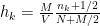
$h_k=\frac{M}{V} \frac{n_k+1/2}{N+M/2}$ .

In the case of a normal distribution the authors suggest a sample of 150 data points to “accurately and consistently estimate the shape of the distribution”.

The following figure shows the relative log-posterior of the number of bins (left) and the estimated histogram for a mixture of three normal samples and a uniform [0,50] (right).

Knuth, K. H. (2013). Optimal data-based binning for histograms. arXiv preprint physics/0605197. The first version of this paper was published on 2006.

Jones, M. C., Marron, J. S., and Sheather, S. J. (1996). A brief survey of bandwidth selection for density estimation. Journal of the American Statistical Association,91(433), 401–407.

Journal club: Half a century of Ramachandran plots

In last week’s journal club we delved into the history of Ramachandran plots (Half a century of Ramachandran plots; Carugo & Djinovic-Carugo, 2013).

Polypeptide backbone dihedral angles. Source: Wikimedia Commons, Bensaccount

50 years ago Gopalasamudram Narayana Ramachandran et al. predicted the theoretically possible conformations of a polypeptide backbone. The backbone confirmations can be described using three dihedral angles: ω, φ and ψ (shown to the right).

The first angle, ω, is restrained to either about 0° (cis) or about 180° (trans) due to the partial double bond character of the C-N bond. The φ and ψ angles are more interesting, and the Ramachandran plot of a protein is obtained by plotting φ/ψ angles of all residues in a scatter plot.

The original Ramachandran plot showed the allowed conformations of the model compound N-acetyl-L-alanine-methylamide using a hard-sphere atomic model to keep calculations simple. By using two different van der Waals radii for each element positions on the Ramachandran plot could be classified into either allowed regions, regions with moderate clashes and disallowed regions (see Figure 3 (a) in the paper).

The model compound does not take side chains into account, but it does assume that there is a side chain. The resulting Ramachandran plot therefore does not describe the possible φ/ψ angles for Glycine residues, where many more conformations are plausible. On the other end of the spectrum are Proline residues. These have a much more restricted range of possible φ/ψ angles. The φ/ψ distributions of GLY and PRO residues are therefore best described in their own Ramachandran plots (Figure 4 in the paper).

Over time the Ramachandran plot was improved in a number of ways. Instead of relying on theoretical calculations using a model compound, we can now rely on experimental observations by using high quality, hand picked data from the PDB. The way how the Ramachandran plot is calculated has also changed: It can now be seen as a two-dimensional, continuous probability distribution, and can be estimated using a full range of smoothing functions, kernel functions, Fourier series and other models.
The modern Ramachandran plot is much more resolved than the original plot. We now distinguish between a number of well-defined, different regions which correlate with secondary protein structure motifs.

Ramachandran plots are routinely used for structure validation. The inherent circular argument (A good structure does not violate the Ramachandran plot; The plot is obtained by looking at the dihedral angles of good structures) sounds more daring than it actually is. The plot has changed over time, so it is not as self-reinforcing as one might fear. The Ramachandran plot is also not the ultimate guideline. If a new structure is found that claims to violate the Ramachandran plot (which is based on a huge body of cumulative evidence), then this claim needs to be backed up by very good evidence. A low number of violations of the plot can usually be justified. The Ramachandran plot is a local measure. It therefore does not take into account that domains of a protein can exert a force on a few residues and just ‘crunch’ it into an unusual conformation.

The paper closes with a discussion of possible future applications and extensions, such as the distribution of a protein average φ/ψ and an appreciation of modern web-based software and databases that make use of or provide insightful analyses of Ramachandran plots.

From Protein Interface Recognition to Protein Complex Prediction

Similarly to ‘words’, which need to be “assembled into sentences, paragraphs, chapters and books” to tell a story, ‘protein structures’ need to be assembled into protein complexes to perform a specific task. To form complexes, proteins interact with other proteins, DNA, RNA and small molecules using their interface residues. All those types of interactions are under intense scrutiny by the research community, each of them defining a distinct field of research. During my PhD I focused on protein-protein interactions (PPIs) and prediction of their interfaces. Modifications in PPIs affect the events that take place within cells which may lead to critical diseases such as cancer. Therefore, knowledge about PPIs and their resulting 3D complexes can provide key information for drug design.

Docking is a popular computational method which predicts the possible structure of the complex produced by two proteins using the known 3D structure of the individual proteins. However, docking of two proteins can result in a large number of different conformational models whose majority is far from correct. This highlights one of the main limitations of docking. Therefore, scoring functions have been proposed which are used to re-score and re-rank docked conformations in order to detect near-native models. One way to distinguish native-like models from false docked poses is to use knowledge of protein interfaces. If one knows the possible location of interface residues on each individual protein, docked complexes which do not involve those interfaces can be rejected. Therefore, accurate prediction of protein interfaces can assist with detection of native-like conformations.

Various methods have been proposed for predicting protein interfaces as mentioned above. A high number of methods investigate protein sequential or structural features in order to characterise protein interfaces. Usage of 3D structural properties has improved the sequence-based predictions. Moreover, evolutionary conservation was shown to be an important property. Therefore, methods have integrated various structural features along with evolutionary information to increase performance.

The combination of different features using various techniques has been investigated by intrinsic-based predictors. However, it seems that these methods have reached their saturation, and combination of more properties does not improve their prediction performance. On the other hand, many studies have investigated the 3D structure of binding sites among protein families. They discovered that the binding site localisation and structure are conserved among homologous. These properties have improved the detection of functional residues and protein-ligand binding sites. Therefore, predictors took advantage of structurally conserved residues among homologous proteins to improve binding site predictions.

Although homologous template-based predictors improve the predictions, they are limited to those proteins whose homologous structure exists. Therefore, methods have extended their search for templates to structural neighbours, since interface conservation exists even among remote structural neighbours. In addition, with the increase in experimentally determined 3D complexes good quality templates can be found for many proteins. Therefore, usage of structural neighbours is the current focus of template-based protein interfaces predictors.

Although, template-based methods are currently the predictors under the main focus, one of their main limitations is their dependency to availability of the QP 3D structure. Also, these predictors have not investigated the contribution of interacting partners of structural neighbours in the prediction. In addition, since these methods perform structural comparisons their computational time is high which limits their application to high-throughput predictions.

One of my PhD contributions was toward developing, T-PIP (Template based Protein Interface Prediction), a novel PIP approach based on homologous structural neighbours’ information. T-PIP addresses the above mentioned limitations by quantifying, first, homology between QP and its structural neighbours and, second, the diversity between the ligands of the structural neighbours (here, ligands refers to the interacting partners of proteins). Finally, predictions can be performed for sequences of unknown structure if that of a homologous protein is available. T-PIP’s main contribution is the weighted score assigned to each residue of QP, which takes into account not only the degree of similarity between structural neighbours, but also the nature of their interacting partners.

In addition, we used T-PIP prediction to re-rank docking conformations which resulted in T-PioDock (Template based Protein Interface prediction and protein interface Overlap for Docking model scoring), a complete framework for prediction of a complex 3D structure. T-PioDock supports the identification of near-native conformations from 3D models that docking software produced by scoring those models using binding interfaces predicted by T-PIP.

T-PioDock Pipeline

Exhaustive evaluation of interface predictors on standard benchmark datasets has confirmed the superiority of template base approaches and has showed that the T-PIP methodology performs best. Moreover, comparison between T-PioDock and other state-of-the-art scoring methods has revealed that the proposed approach outperforms all its competitors.

Accurate identification of near-native conformations remains a challenging task. Although availability of 3D complexes will benefit to template based methods such as T-PioDock, we have identified specific limitations which need to be addressed. First, docking software are still not able to produce native like models for every target. Second, current interface predictors do not explicitly refer to pair-wise residue interactions which leaves ambiguity when assessing quality of complex conformations.

Network Analysis

Why networks?

Individual expression could be thought as a phenomenon regulated mostly by the individual, but in a second stand it is also modified by the interactions with the surroundings. Can the response of the individual be predicted by the group? (See the following video of an experiment conducted by Asch https://www.youtube.com/watch?v=FnT2FcuZaYI)

networkinside

Most common type of network analysis

Basic network summary statistics (description)
Clustering methods (Extract information)
Random graphs (Description, inference and to model network topology)
Learning machine methods (Prediction)

Random Graphs and the topology structure

Depending on the structure of a desired network different random models could be of use, for example, if the goal is to obtain a sparse and not highly connected network then an ER model could be of use (this model randomly assign the edges between nodes)

or if the goal is exactly the opposite (have a very highly connected network) a geometric graph could be of use (this model randomly assign positions in a n-dimensional space and then place edges between nodes closer than a given distance).

Is there already a random model?

According to our recent results we suspect there is no null model yet for PPIs, even though for some virus PPIs some of the random models seem to be very good models; however this virus PPIs are much smaller (around 300 nodes and up to 500 edges) than the networks of model organisms (usually with more than 2000 nodes and 5000 edges) such as yeast, human, fruit fly and Escherichia coli among others.

We will soon be publishing our article with details about this.

Django for scientific applications

In my current work I am developing a cheminformatics tool using structural and activity data to investigate protein-ligand binding. I ~~have only ever properly used~~ love python and I listen to Saulo, so I decided to used Django to develop my application. I didn’t understand what it was and why it might be useful before I started using it but below I thought I’d discuss a few of the features that I think have been useful and might encourage others to use it.

Firstly I will outline how Django works. I wanted to download all the PDB structures for CDK2 and store the information in a data structure that is robust and easily used. We have a Target and a Protein. A Target is associated to a particular UniProt accession. Cyclin-dependent kinase 2 (CDK2) is a Target. A Protein is a set of 3D coordinates, so 1AQ1 is a Protein.

class Target(models.Model):
"""A Django model to define a given protein target"""
    UniProt = models.CharField(max_length=20,unique=True)
    InitDate = models.DateTimeField(auto_now_add=True)
    Title = models.CharField(max_length=10)

In the above Target model I have three different fields. The first field denotes the UniProt accession for the Target and is “unique”. This means that only one Target can have any given UniProt accession in my data structure. If I try to add another with the same value in the UniProt field it will throw an exception. The second field denotes the time and date that the model was created. This means I can check back to when the target was created. The third is the Title I would like to use for this, for example CDK2.

I can then make a new Target objects by:

new_target = Target()
new_target.Title = "CDK2"
new_target.UniProt = "P24941"

and save it to the database by:

new_target.save() # Django takes care of the required SQL

The next model is for the Protein molecules:

class Protein(models.Model):
    """A Django model to define a given protein"""
    Code = models.CharField(max_length=6,unique=True)
    InitDate = models.DateTimeField(auto_now_add=True)
    TargetID = models.ForeignKey(Target)
    Apo = models.BoolenField()
    PDBInfo = models.FileField(upload_to='pdb')

The model contains the PDB Code, e.g. 1AQ1, and the date it was added to the database. It also consists of a foreign key, relating it to its Target and a boolean indicating if the structure is apo or holo. Finally there is a file field relating this entry to the appropriate file path where the PDB information is stored.

Once the data has been added to the database, Django then deals with all SQL queries from the database:

my_prot = Protein.objects.get(Code="1aq1") # Gives me the Protein object "1aq1"
CDK2_prots = Protein.objects.filter(TargetID__Title="CDK2") # All PDB entries associated to CDK2, as a query set, behaving similarily to a list
CDK2_list = [x for x in CDK2_prots] # Now exactly like a list

The “__” in the above query allows one to span the foreign key relationship, so it is searching for the Title of the Target not the Title of the Protein. Finally I can then access the PDB files for each of these proteins.

my_prot = Protein.objects.get(Code="1aq1") # Gives me the Protein object "1aq1"
print my_prot.Code # prints "1aq1"
# my_prot.PDBInfo has the behaviour of a file handle
pdb_lines = my_prot.PDBInfo.readlines()# Reads the lines of the file

There, you’ve made a queryable database, where Django deals with all the hard stuff and everything is native to python. Obviously in this example it might not be so difficult to imagine alternative ways of creating the same thing using directory structures, but as the structure of your data becomes more complex, Django can be easily manipulated and as it grow it utilises the speed advantages of modern databases.

A very long introductory post about protein structure prediction

If you are a protein informatician, bioinformatician, biochemist, biologist or simply a person well informed about science, you probably heard about protein structure prediction. If that is the case, you might be wondering what all the fuss is about, right? If you never heard those terms before, don’t panic! You are about to find out what protein structure prediction is all about!

Based on my group meeting’s presentation last Wednesday, this blog entry will discuss why protein structure prediction is important and the potential limitations of existing methods. I will also discuss how the quality of input may be a potential source for lack of accuracy in existing software.

First, let us remember a little biology: our genetic code encrypts the inner-works of a complicated cellular machinery tightly regulated by other (macro)molecules such as proteins and RNAs. These two types of macromolecules are agents that perform the set of instructions codified by DNA. Basically, RNAs and proteins are involved in a series of processes that regulate cellular function and control how the genetic code is accessed and used.

For that reason, a huge chunk of genomic data can be ~~pretty useless~~ not that useful if considered on their own. Scientists around the globe have invested millions of moneys and a huge chunk of time in order to amass piles and piles of genome sequencing data. To be fair, this whole “gotta sequence ’em all” mania did not provide us with the fundamental answers everybody was hoping for. Cracking the genetic code was like watching an episode of Lost, in which we were left with more questions than answers. We got a very complicated map that we can’t really understand just yet.

For that reason, I feel obliged to justify myself: protein structures ARE useful. If we know a protein structure, we can formulate a very educated guess about that protein’s function. Combine that with empirical data (e.g. where and when the protein is expressed) and it can help us unveil a lot of info about the protein’s role in cellular processes. Basically, it can answer some of the questions about the (genomic) map. ~~If only we could do that with Lost…~~

There is also evidence that knowing a protein’s structure can help us design specific drugs to target and inhibit that protein. Although the evidence of such biomedical application is sparse, I believe that with development of the field, there is a trend for protein structures to become more and more important in drug discovery protocols.

Still, if we look at the number of known genome sequences and known protein structures and at the growth of those figures over the past decade, we look at a drastic scenario:

There is a tendency for the gap between the number of protein sequences and protein structures to increase. Hence, we are getting more and more questions and little to no answers. Observe how the green line (the protein sequences associated with a known or predicted function) is very close to the red line (the number of known protein structures). However, there is a growing gap between the red and the blue line (the number of protein sequences). Source: http://gorbi.irb.hr/en/method/growth-of-sequence-databases/

Well, gathering protein structure data is just as important, if not more important, than gathering sequence data. This motivated the creation of Structural Genomics Consortiums (SGC), facilities that specialize in solving protein structures.

I am sorry to tell you that this is all old news. We have known this for years. Nonetheless, the graph above hasn’t changed. Why? The cost limitations and the experimental difficulties associated with protein structure determination are holding us back. Solving protein structures in the lab is hard and time consuming and we are far from being as efficient at structure determination as we are at genome sequencing.

There is a possible solution to the problem: you start with a protein sequence (a sequential aminoacid list) and you try to predict its structure. This is known as protein structure prediction or protein structure modelling. Well, we have a limited number of building blocks (20) and a good understanding of their physicochemical properties, it shouldn’t be that hard right?

Unfortunately, modelling protein structure is not as simple as calculating how fast a block slides on an inclined plane. Predicting protein structure from sequence is a very hard problem indeed! It has troubled a plethora of minds throughout the past decades, making people lose many nights of sleep (I can vouch for that).

We can attribute that to two major limitations:

1- There are so many possible ways one can combine 20 “blocks” in a sequence of hundreds of aminoacids. Each aminoacid can also assume a limited range of conformations. We are looking at a massive combinatorial problem. The conformational space (the space of valid conformations a protein with a given sequence can assume) is so large that if you could check a single conformation every nanosecond, it would still take longer than the age of the universe to probe all possible conformations.

2- Our physics (and our statistics) are inaccurate. We perform so many approximations in order to make the calculations feasible with current computers that we end up with very inaccurate models.

Ok! So now you should know what protein structure prediction is, why it is important and, more importantly, why it is such a hard problem to solve. I am going to finish off by giving you a brief overview of the two most commons approaches to perform protein structure prediction: template-based modelling (also known as homology modelling) and de novo structure prediction.

There is a general understanding that if two proteins have very similar sequences (namely, if they are homologs), than they will have similar structures. So, we can use known structures of homologs as templates to predict other structures. This is known as homology modelling.

One can do a lot of fancy talk to justify why this works. There is the evolutionary argument: “selective pressure acts on the phenotype level (which can encompass a protein structure) rather than the genotype level. Hence protein structures tend to be more conserved than sequence. For that reason and considering that sequence alone is enough to determine structure, similar sequences will have even more similar structures.”

One can also formulate some sort of physics argument: “a similar aminoacid composition will lead to a similar behaviour of the interacting forces that keep the protein structure packed together. Furthermore, the energy minimum where a certain protein structure sits is so stable that it would take quite a lot of changes in the sequence to disturb that minimum energy conformation drastically.”

Probably the best argument in favour of homology modelling is that it works somewhat well. Of course, the accuracy of the models has a strong dependency on the sequence similarity, but for proteins with more than 40% identity, we can use this method in order to obtain good results.

This raises another issue: what if we can’t find a homolog with known structure? How can we model our templateless protein sequence then? Well, turns out that if we group proteins together into families based on their sequence similarity, more than half of the families would not have a member with known structure. [This data was obtained by looking at the representativeness of the Pfam (a protein family database) on the PDB (a protein structure database).]

Ergo, for a majority of cases we have to perform predictions from scratch (known as free modelling or de novo modelling).

Well, not necessarily from scratch. There is a specific approach to free modelling where we can build our models using existing knowledge. We can use chunks of protein, contiguous fragments extracted from known structures, to generate models. This is known as a fragment-based approach to de novo protein structure prediction. And that is one big name!

One can think of this as a small scale homology modelling, where both the physics and evolutionary arguments should still hold true to some degree. And how do we do? Can we generate good models? We perform appallingly! Accuracies are too low to generate any useful knowledge in a majority of cases. The problem with the rare cases when you get it right is that you have no means to know if you actually got the right answer.

The poor quality of the results can be justified by the 2 biggest limitations discussed above. Yet something else might be in play. In homology modelling, if you use a bad template, you will most certainly get a bad model. In a similar way, using a bad set of fragments will lead you to a very poor final model.

Considering we already have the other two big issues (size of conformational space and accuracy of current potentials) to worry about, we should aim to use the best fragment library we possibly can. This has been the recent focus of my work. An attempt to make a small contribution to solve such a hard problem.

I would love to detail my work on finding better fragments here, but I believe this post is already far too long for anyone to actually endure it and read it until the end. So, congratulations if you made it through!

Oxford Protein Informatics Group

or "OPIG" to friends