
As it’s known in non-parametric kernel density estimation the effect of the bandwidth on the estimated density is large and it is usually the parameter who makes the tradeoff between bias and roughness of the estimation (Jones et.al 1996). An analogous problem for histograms is the choice of the bin length and in cases of equal bin lengths the problem can be seen as finding the number of bins to use. A data-base methodology for building equal bin-length histograms proposed by (Knuth 2013) based on the marginal of the joint posterior of the number of bins and heights of the bins. To build the histogram first the number of bins has to be selected as the the value (

where 


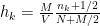
Now, the height (
In the case of a normal distribution the authors suggest a sample of 150 data points to “accurately and consistently estimate the shape of the distribution”.
The following figure shows the relative log-posterior of the number of bins (left) and the estimated histogram for a mixture of three normal samples and a uniform [0,50] (right).

Knuth, K. H. (2013). Optimal data-based binning for histograms. arXiv preprint physics/0605197. The first version of this paper was published on 2006.
Jones, M. C., Marron, J. S., and Sheather, S. J. (1996). A brief survey of bandwidth selection for density estimation. Journal of the American Statistical Association,91(433), 401–407.