Tag Archives: protein structure

Augmented Modelling with Natural Move Monte Carlo Simulations

In the last group meeting I reported on the progress that I have made regarding the development of a protocol for the systematic use of Natural Move Monte Carlo simulations.

Natural Move Monte Carlo simulations
Natural Moves are degrees of freedom that describe the collective motion of groups of residues. In DNA this might be the concerted motion of a double helix; in proteins this could be the movement of a stable secondary structure element such as a beta-sheet. These segments are joined by so called melting areas. At each simulation step the segments are propagated independently in an MC fashion. The resulting chain breaks are resolved by a chain closure algorithm that acts on the melting areas. This results in a reduction of degrees of freedom of several orders of magnitude. Therefore, large complexes and conformational changes can be sampled more effectively.

In order to get sensible results, however, the initial decomposition of the system is important. The challenge is to accurately represent the plasticity of the system, while keeping the number of degrees of freedom as small as possible. Detailed insight into the flexibility of the system might be gained from experimental sources such as NMR or computational methods such as MD simulations and Normal Mode Analysis. This can help with defining segments and melting areas. However, there are many systems for which this data is not available. Even if it is, there is no guarantee that the segmentation is correct.

Therefore, I am developing a protocol that allows for the evaluation of a range of different test cases that each reflect a unique set of segments and melting areas.

Augmented Modelling Protocol
This protocol is aimed at the systematic evaluation of NMMC segmentations. It allows researchers to feed experimental information, biological knowledge and educated guesses into molecular simulations and so provides a framework for testing competing hypotheses. The protocol has four steps.

Step 1: Segmentation of the system into low-level segments
The initial segmentation contains all possible areas of flexibility that may play a role in conformational changes in the system of interest. This decision may be influenced by many sources. For now, however, we only consider secondary structure information. Helices and beta strands are treated as potential segments. Unstructured regions such as kinks, loops and random coils are treated as melting areas. For a small fold with four helices we get the segmentation shown in figure 1a.

Step 2: Formulate test cases
Generate multiple test cases that reflect hypotheses about the mechanism of interest. In this step we try to narrow down the degrees of freedom as much as possible in order to retain sampling efficiency. This is done by selectively deactivating some melting areas that were defined in step 1. For a system with three melting areas that can either be on or off, 2^3 = 8 different test cases may be generated (example shown in figure 1b).

Figure 1 a) Segmentation of a small α-fold. The blue rectangles represent α-helices. The dashed lines indicate the presence of melting areas I, II and III. Each melting area can be switched on or off (1/0) b) Example of a test case in which the first of three melting area is switched off. c) The six degrees of freedom along which a segment is propagated.

Step 3: Perform simulations
Sample the conformational space of all test cases that were generated in step 2. We generally use Parallel Tempering or Simulated Tempering algorithm to accelerate the sampling process. These methods rely on the modulation of temperature to overcome energy barriers.

Step 4: Evaluate results
Score the results against a given control and rank the test cases accordingly. The scoring might be done by comparing experimental distributions of observables with those generated by simulations (e.g. Kullback-Leibler divergence). A test case that reproduces desired expectation values of observables might then be considered as a candidate hypothesis for a certain structural mechanism.

What’s next?
I am currently working on example uses for this protocol. These include questions regarding aspects of protein folding and the stability of the empty MHC II binding groove.

de novo Protein Structure Prediction software: an elegant “monkey with a typewriter”

In this week’s OPIG group meeting, I discussed the inner-works and the algorithm behind ROSETTA, one of the most well-known software for de novo protein structure prediction.

Before we even attempt to understand how ROSETTA works, let us start with a theorem.

Theorem: given an infinite number of monkeys with typewriters and an infinite amount of time, they are very likely to recreate the works of William Shakespeare.

Monkey with a typewriter… Time to write that Shakespeare!

Well, let us be a little more modest and attempt to recreate just a phrase of old Bill, instead of his whole works:

“The fool doth think he is wise, but the wise man knows himself to be a fool.”

Well, if we exclude spaces and punctuation marks, that leaves us 58 positions in our phrase (the length of the quote). Considering we have 26 possible letters for each position, we would expect to generate this phrase at random once every of 26^58 times. Wow!

That means that we need to evolve from monkeys (pun intended) and appeal to our over-developed encephalon!

In order to steer our Monkey typewriter, we can reduce this problem to a Global Optimisation problem. In a Global Optimisation problem, we define a function f (named an objective function) which we want to minimise for a given set of parameters x. Bare in mind that if we want to maximise a given function f, we can define g = -f

In a global optimisation problem, we are interested in finding the values of X that minimise the function f(X).

Now, all we need is to define an objective function in order to guide our Monkey typewriter towards the right answer.

Let us define the following objective function: given our Shakespearean phrase and a sequence of 58 letters, the value of the objective function equals the number of letters that are different between the phrase and the sequence of letters.

We can now proceed to define a slightly more refined Monkey Typewriter:

1- Start with a random sequence of letters.
2- WHILE sequence != shakespearean_phrase:
3-________ Select a random position in the sequence.
4-________ Assign a new letter to that position.
5-________ IF score of new sequence < score of old sequence:
6-__________________ Accept the change.
7-________ ELSE:
8-__________________ Discard the change.

This way we can steer our Monkeys and reduce the time it would take to generate our Shakespearean phrase to a more feasible time.

Now, let’s talk about protein structure prediction (PSP). More specifically, let us talk about de novo protein structure prediction (different flavours of protein structure prediction have been discussed previously here).

One of the great ideas behind the creators of ROSETTA, was to use a combination of two different techniques to address the big problems of protein structure prediction:

1- Problem number #1 of PSP is the size of the conformational space. A protein can be represented by it’s backbone atoms, which, in turn, can be reconstructed from a sequence of torsion angles. A set of 3 torsion angles can be used to represent every protein residue. Therefore, for a protein with 100 residues, we would have a total of 300 angles. If we approximate each angle to assume one of 360 values (degrees), that gives us 360^300 possible conformations (not huge at all, han?).

One of the main ideas behind ROSETTA was to reduce the search space by using fragments extracted from known structures. The use of fragments restricts the possible angles to a set of values that are known to occur in nature. Therefore, instead of looking at 360^300 possible angles, we deal with a much more feasible search space.

The name ROSETTA is based on the Rosetta Stone, an archaeological artefact that allowed modern civilisation to interpret and convert between different alphabets. In reality, ROSETTA can be seen as a very elegant monkey typewriter. ROSETTA uses sequence and structure similarity to define a structural alphabet. For every single position in our protein sequence, we have a set of fragments extracted from now protein structures to represent that position. Originally, each position would be represented by 25 fragments (letters?). If you combine the different pieces of known structures in the right order, you will get your Shakespearean Phrase in the end (the correct Protein Structure!).

2- Well, we still have a pretty big conformational space considering we have 25 fragments per position (approximately 25^100 possible conformations, for a protein with 100 residues). The second technique employed by ROSETTA is Simulated Annealing.

Simulated Annealing is a Global Optimisation heuristic. It attempts to find a good enough solution to the problem of minimising a given function f. It is very similar to our Monkey Typewriter algorithm. The main difference is that Simulated Annealing implements some tricks to avoid local minima entrapment. In simpler terms, if we ONLY accept favourable changes (Line 5 of Monkey Typewriter pseudo-code), once we reach a local minimum, we get trapped. No possible change would lead to an improvement, yet we are still far from finding the global minimum.

In order to mitigate that entrapment effect, Simulated Annealing defines a probability of accepting an unfavourable change. This probability is higher at the beginning of the simulation and it becomes lower and lower as the simulation progresses. This process is usually referred to as “cooling down”.

Ok! So we reduced our PSP problem to an elegant Monkey Typewriter. We have our Monkeys working to create the best possible Shakespeare, in a pretty clever and sophisticated manner. Well, we should be able to create some fine piece of literature, correct?

Not quite!

There are still several problems with this whole pipeline. I will mention a few:

When you define your structural alphabet, you may not have the right fragment to represent a certain position. This would be the same as trying to get to a Shakespearean phrase without using vowels for the first 10 letters or only using consonants in the middle of the sentence. It would never happen…
Despite the many efforts to define a very good objective function, no current software presents a function that truly mimics the behaviour of an energy function. This implies that we have a vague idea of how the Shakespearean phrase should look like, but we cannot precisely pinpoint where each letter goes.
No matter how elegant our Monkey typewriter becomes, the combinatorial problem still persists. We are still dealing with 25^100 possible conformations and it is impossible to try every single conformation.
The objective function, if plotted in a graph, would look completely hideous (unlike the picture above). We are talking about a gigantic multi-dimensional surface, filled with local minima that confuse and entrap our simulations. Combine that with the fact that our objective function is not accurate and you waste most of your computing power into generating solutions that are completely useless.
Another common technique to address the previous limitations is to increase the number of Monkeys in order to speed up the search process. If you use thousands and thousands of Monkeys (multiple runs of ROSETTA), each individual Monkey will get to a local minimum (decoy = something that looks like a phrase). In recent years, tens of thousands of decoys are generated in order to predict a single structure. A new problem arises, because out of these tens of thousands of phrases, we cannot tell apart Hamlet from Twilight. We don’t know which Monkeys got close to the right answer. All we know is that for some cases some of them did.

In conclusion, de novo Protein Structure Prediction still has a long way to go.

MAMMOTH: a case study in protein structure alignment

I’ve talked about protein structure alignment before in the context of a rather novel, mathematical approach. This time I wanted to revisit the topic in a general sense, using a more established algorithm as a case study. MAMMOTH stands for Matching Molecular Models Obtained from Theory and was first published in 2002. Since then it has been cited nearly 400 times and the underlying algorithm has been extended to a multiple alignment program: MAMMOTH-mult.

Establishing biologically relevant and consistent alignments between protein structures is one of the major unsolved problems in computational bioinformatics. However, it’s an important part of many challenges that we face: such as establishing homology between distantly related proteins, functional inference for unannotated proteins, and evaluating the accuracy of models of predicted structure for competitions such as CASP.

Problem Outline

In essence the problem of protein structure alignment can be outlined by considering two ordered sets of coordinates, A = {a₁,a₂,…,a_n} and B = {b₁,b₂,…,b_m}, representing points in 3D space. In most cases these points will be the location of the C_α atoms along each structure’s backbone. The sets A and B might be completely different lengths and, if an alignment exists, are almost certainly orientated differently compared to each other.

Establishing an alignment between these sets is equivalent to two steps:

Establish a match M = {(a_i,b_j) | a_i ∈ A, b_j ∈ B}
Rotate and translate A onto B so that equivalent atoms are as close as possible.

Of course, it is not immediately clear how to best fulfill these requirements. In particular, we don’t really know what features to prioritise for a biologically relevant match. Should we try to match secondary structure elements and what penalty should we attach to mismatched elements? How about maintaining the correct hydrogen bonding patterns between matched residues? And how much weight should we put on the matched atoms being consecutive in each set (i.e. how should we penalise gaps)?

The second step is equally ambiguous. Especially as there is no consensus on what the correct interpretation of close is. Minimising the RMSD between equivalent atoms is a popular choice of distance measure. However, as the MAMMOTH paper points out, RMSD is often dominated by the mismatched portions of remotely related structures and is thus largely inappropriate in these cases. Furthermore, even if we have a well-defined distance metric, should the superposition prioritise minimising the distances between nearly identical parts of the different structures, at the expense of less similar substructures? Or should the emphasis be on maintaining as lengthy a match as possible at the possible cost of a lower closeness of fit? How about the relative importance of a close fit for atoms in the core of the structure vs. those on the surface?

The majority of these questions remain unanswered and as a result it is often hard to validate alignments as we simply do not know what the right answer is. In fact, in many cases, manual analysis is preferred over any of the available computational techniques.

In this post I’ll go through how the MAMMOTH algorithm approaches each of these steps. For many of the above questions MAMMOTH does not postulate a solution, primarily because, as its name suggests, it was designed to assess prediction models which are often at low resolutions and lacking secondary structure or hydrogen bonding information. I think it’s important to keep these questions in mind, but there’s certainly no necessity to design a programme which deals with them all.

Step 1: Pairing up residues (similarity matrix)

In order to establish a match between equivalent atoms in A and B, MAMMOTH, like several other structural alignment algorithms, uses a well-established alignment technique: a similarity matrix (often inferred from and referenced as a distance matrix). A similarity matrix for alignment is an n x m array where each entry S(a_i,b_j) represents the pairwise similarity score between residues a_i and b_j. An alignment between the residues of A and B is any non-decreasing path (that is, a pair (a_i,b_j) in the path must appear later in the ordering of coordinates of both A and B than the preceding pair of residues in the path) from the top left corner of the array (a₁,b₁) to the bottom right corner (a_n,b_m). For example the following path can be interpreted as an alignment between A = {a₁, …, a₁₁} and B = {b₁, …, b₈}

Any alignment can be scored by summing up the similarity scores along this path, while penalising any gaps in an appropriate way (normally, these algorithms use trial and error to decide on sensible penalties). For example, the above alignment would have the score S = S(a₁,b₁) + S(a₂,b₂) + S(a₃,b₃) + S(a₇,b₄) + S(a₈,b₅) + S(a₉,b₆) + S(a₁₀,b₇) + S(a₁₁,b₈) + α + 2β, where α and β are gap opening and gap extension penalties respectively. The optimal alignment is simply the alignment which maximises this score.

For sequence alignments similarity scores can be assigned to residues from substitution tables like BLOSUM. However, it is not immediately clear of an appropriate equivalent for structures. MAMMOTH, like several other algorithms, defines the similarity between different residues by examining their local structural landscape. Specifically, this means comparing fragments of each backbone, centred on the residue of interest. MAMMOTH uses the URMS distance between heptapeptide fragments. This distance is illustrated below using 2D chains and tripeptide fragments.

Comparing residues a₂ and b₃ involves looking at the directions between each successive residue of the fragment. Each vector is mapped to the unit sphere, beginning at the origin and ending at the surface of the sphere (in this case 2 vectors are considered, and in MAMMOTH’s case 6 different 3D vectors are mapped). The optimal rotation is found, superposing equivalent vectors as best as possible, and then the RMSD of the endpoints on the surface of the sphere is calculated as URMS(a_i,b_j).

Aside: The optimal superposition of a set of vectors is actually a non-trivial problem. It is essentially equivalent to step 2 in our alignment protocol outlined above, but is significantly easier for the 6 vectors characterising a fragment in MAMMOTH’s algorithm.

Finally, S(ai,bj) is calculated by converting the distance into a similarity measure:

where URMS^R is the expected URMS of a random set of vectors and:

The optimal alignment through this MAMMOTH matrix is the path which maximises the sum of similarities between matched residues (each residue being at the centre of the heptapeptide fragment) using gap opening and extension penalties of 7.00 and 0.45 respectively.

Step 2: Global superposition (MaxSub)

The above alignment results in a match M’ optimising the local structural similarity of residues in each structure, however, their is no guarantee that this will result in a set of coordinates close in global space. In order to finalise the match set M ⊆ M’ as well as calculating the optimal superposition of the paired residues of A onto their equivalent points in B, MAMMOTH use the MaxSub algorithm. This is a very efficient algorithm (worth a read if you’re that way inclined) for calculating the maximal subset from a set of paired up atoms which are close in global space. MAMMOTH decide that close means < 4A away after superposition. They do not try to optimise a closer superposition than that but attempt to find the largest possible set of matched residues.

The MaxSub algorithm relies on the assumption (made for computational tractability) that the final subset M ⊆ M’ will have, somewhere, a set of at least four residues consecutive in M’. The algorithm then starts with every possible seed of four consecutive residues (just to illustrate the power of the assumption in reducing computational time: for a 150 residue protein there are just 147 such seeds, but over 2 million sets of four non-consecutive residues!! And it’s a pretty reasonable assumption to make as well). The MaxSub algorithm then calculates the superposition for those four matched pairs, extending the set of residues that are <4A away from their partners, recalculating the superposition using these new pairs as well, then removing any pairs which are no longer within the threshold of each other. It repeats these steps, gradually extending the set M, until the algorithm converges.

Scoring the alignment

Using the two approaches outlined above, MAMMOTH generates an alignment between the two input structures. In order to summarise the significance of this alignment, the algorithm generates the PSI score: the percentage structural identity (which is simply the size of the maximum subset divided by the length of the shortest protein). As a global measure of the strength of similarity the PSI score is poorly constructed and scales with protein length. In order to adjust for this bias, MAMMOTH fits a Gumbel distribution to PSI scores obtained from random structure comparisons between unrelated proteins at bins of different lengths. This results in a z-score measuring, instead of the PSI of an alignment, the likelihood of obtaining a PSI score as good as that by chance between any two proteins of the same lengths.

Journal Club: Native contacts in protein folding

Like your good old headphone cables, strings of amino acids have the potential to fold into a vast number of different conformations given the appropriate conditions. A conservative estimation for the time it would take a 100 residue protein to explore all theoretically possible conformations would exceed the age of the Universe several times. This is obviously not feasible and was pointed out by Levinthal when he published his “How To Fold Graciously” in 1969.

The so called Protein-Folding Problem has since been under intense study, which inevitably has led to a few theories and models about its nature. Due to the lack of appropriate wet-lab methods to study this phenomenon theoretical, computational approaches have been key to devising impactful frameworks for formally describing protein folding. One of these goes under the name of principle of minimum frustration introduced by Bryngelson and Wolynes in the late 80s (1). It states that proteins by evolution were enriched for sequences with the propensity to fold into low-energy structures, while actively selecting against traps. By avoiding mis-folding and non-native contacts, the theory says, a smooth funnel-like energy landscape with native-state minima is created that ensures robust and fast folding.

This implies that native contacts, i.e. residues that interact in the fully folded protein play a major role in the folding process. Gō models (2), named after Nobuhiro Gō who first proposed this method, are based around this assumption with the energetic contributions of native interactions acting as the sole driving forces in the folding process. While this approach has yielded promising results, many of which were in concordance with experiments, its underlying principles have never been validated in a statistically meaningful way.

A schematic for native-contact-driven protein folding

In 2013 a study by Best, Hummer and Eaton (3) formally addressed this question. By devising a set of statistical quantities aimed at weighting the importance of native and non-native interactions for folding and applying these to the analysis of several long MD folding simulations they were able to show a “native-centric mechanism” for small fast-folding proteins.

In a first step it was assessed whether the fraction of native contacts provided a suitable reaction coordinate for the simulated folding events. From their equilibrium simulations two thresholds of native-contact-fractions were chosen that defined folded and unfolded states (a two-state model is assumed). Overlaying the values for the most visited native-contact-fractions during simulation against these thresholds revealed a strong correlation between the two equilibrium probability density maxima and the protein’s fold state. In addition they showed that the range of native-contact-fractions between those found to represent unfolded and folded thresholds were indicative of being on a transition path (defined as the “.. regions of the trajectories that cross directly from the unfolded well to the folded well ..”).

A further measure was introduced with the contact lifetime test. The log-ratio of the time a contact spent on a transition path vs the time it existed in the unfolded state was calculated and compared in a heat-map to the native contact map coloured by the number of contacts between residues.

Contact life time test for a selected protein.
Adapted from (3).

Among others this result revealed a clear connection between contacts with longer transition path life times and the number of contacts they made in the native structure.

So what about non-native interactions?

Screenshot from 2014-03-27 12:47:04

One of the measures addressing this question was the Bayesian measure for non-native contacts on transition paths. In the examples used in this paper, no obvious link between being on a transition path given a non-native contact was found unless they were close to native contacts. Further criteria such as the complementary quantity, which is the probability of being on a transition path when a contact is not made, concluded in a similar fashion.

Interestingly, it was found that the one protein that was influenced by non-native contacts was the designed α3D. Best et al. reasoned that additional frustration introduced when building a protein with artificially introduced stability has led to a shifting of helix register giving rise to this outlier.

When taken together, these results lay a robust foundation for further studies along the same lines. It is too early to accept or reject the presented findings as universal truth, but strong arguments for the native-centric mechanism being a reasonable model in small fast-folding proteins have been made. It would not be far-fetched to think that larger proteins would adhere to similar principles with non-native contacts modulating the landscape, especially when considering individual downhill folding modules.

References:

(1) Bryngelson, J.D. et al., 1995. Funnels, pathways, and the energy landscape of protein folding: a synthesis. Proteins, 21(3), pp.167–95.

(2) Taketomi, H., Ueda, Y. & Gō, N., 1975. Studies on protein folding, unfolding and fluctuations by computer simulation. I. The effect of specific amino acid sequence represented by specific inter-unit interactions. International journal of peptide and protein research, 7(6), pp.445–59.

(3) Best, R.B., Hummer, G. & Eaton, W.A., 2013. Native contacts determine protein folding mechanisms in atomistic simulations. Proceedings of the National Academy of Sciences of the United States of America, 110(44), pp.17874–9.

Kinetic Modelling of Co-translational Protein Folding (Journal Club)

Following up on last week’s entry, this post will explore the same topic: polypeptide chains assuming native-like conformations as they are extruded from the ribosome, or for the less intimate with the concept, co-translational protein folding.

Before addressing some important questions concerning co-translational protein folding, I would like to make a parenthesis: I want to dedicate a paragraph or two to talk about time.

Biological processes are dynamic. They are events that occur over a period of time. For instance, one can quantify the effect of mutations propagated and accumulated over millions of years of evolution. One can also quantify the femtoseconds in which subtle conformational changes occur in photoreceptor proteins like rhodopsin, when they respond to light. Time is fundamental to understand and model any sort of biological event.

Albeit it might seem obvious to the reader that time is so crucial to amass biological knowledge, those of us more theoretically inclined (bioinformaticians, computational biologists, biostatisticians, mathematical biologists and so on and so forth) are usually presented with models that tend to over-simplify reality. Surprisingly enough, there are many over-simplistic models that neglect the effect of time in order to “better” represent whatever they claim to model. Take Protein Docking for instance. The biological process at hand presents a complicated dynamic. There is a kinetic equilibrium, in which a vast amount of protein and ligand molecules interact, associating into complexes and dissociating. Nonetheless, Protein Docking is traditionally reduced to the binding affinity between a pair of molecules. As one might say, this is only a problem if I can present a solution… Luckily, Protein Docking is not my subject of expertise, so I will leave this question open to more tenacious minds than my own.

One of the areas in which I am truly interested in is the co-translational aspect of protein folding. If one performs a quick Google Images search, using the terms “Protein Synthesis” or “Protein Translation”, the results tell a very interesting story. The vast majority of nascent protein chains are represented as fully elongates peptide chains. In a majority of pictures, the growing peptides do not even present secondary structure. They are mostly represented by long, unfolded, almost linear polymers.

Now, any first year Biochemistry student learns about something called Hydrophobicity (or hydrophilicity depending on whether you are a glass half empty or half full type of person). It is biochemistry-introductory-text-book stuff that some residues are polar and some residues are apolar, and hence will hide from water, forming a hydrophobic core. That (hydrophobicity) is one of the main driving forces of protein folding.

Hence, most of the images that appear in our Google Images search are not very representative. They are plain wrong. It is simple physics that the growing peptide chains will form secondary and tertiary structures during the process of protein synthesis. One has to remember that this process is dynamic, it is happening over time. Under these circumstances, time should not be neglected. The time scale at which extrusion occurs is slow enough to allow the nascent chain to probe conformations and simply abide to the laws of physics. A fully elongated, completely unfolded and denatured peptide chain would not exist during protein synthesis. These nascent chains would adopt intermediate conformations simply as a result of apolar residues trying to hide from water.

Ok. Now, the BIG question that can be raised is whether those intermediate conformations actually resemble the native state of the fully elongated protein. I do not want to incur in Baby Kicking, but one thing that evolution has taught us is that cells have evolved to be highly efficient systems. There is no room for wasted energy. It makes sense to hypothesize that over millions of years, the cellular machinery has adapted to explore these intermediate conformations in order to make the process of protein folding more efficient.

Over the past couple of years, substantial evidence has been amassed that codon usage and the degeneracy of the genetic code could be exploited by cells to ensure that protein folding occurs accurately and efficiently. There are many theoretical ways that such exploitation could occur: the codon translation speed could facilitate the formation of certain intermediates that are beneficial for protein folding, that increase stability or that prevent protein aggregation. There is even a biomedical impact given that some observed pathologies have been associated with synonymous codon mutations that may lead to misfolded proteins.

In the paper I presented during this journal club [1], O’Brien and colleagues have devised and described a very interesting kinetic model for protein translation. Their model was used to describe possible scenarios in which both fast and slow translation speed codons are coordinators of co-translational protein folding. Please note that, in this context, co-translational protein folding is perceived as an enrichment of intermediate conformations of the nascent chains, which resemble the native structure of the fully elongated protein.

In the model described in the paper, they opted for a probabilistic approach instead of an analytical (differential equations) approach. The time is modelled by the use of probabilities. The authors derived a formula to quantify the expected proportion of nascent chains of a given length that would be in a Folded intermediate state (one that resembles the native structure). They have managed to express this in terms of a rate of codon translation. Therefore, they stablish a direct relationship between Co-Translational protein folding and codon translation speed.

Their analysis is robust as none of the constants and kinetic rates need to be experimentally derived in order to provide insights about the protein folding process. Overall, I think the way the model was built was quite ingenious and very interesting. I would suggest any interested reader to read the article if they want to understand how the whole modelling was carried out.

Overall, I think the authors present a compelling argument for how cells could explore codon degeneracy and co-translational aspects of protein folding to improve folding efficiency. One of their results present a scenario in which fast translation speed codons can be used to assist in the fold of unstable protein regions, preventing the formation of misfolded intermediates.

One of the many functions of mathematical models is to provide insights into the underlying biology of the phenomena they attempt to model. The lack of any experimental evidence to support this paper’s results does not make it any less interesting. The article presents to the readers a sound and solid mathematical argument as to how co-translational aspects of protein folding could be beneficial for cell efficiency. If anything, they provide interesting hypotheses that might drive experimentalists in the future.

[1] Kinetic modelling indicates that fast-translating codons can coordinate cotranslational protein folding by avoiding misfolded intermediates.

A very long introductory post about protein structure prediction

If you are a protein informatician, bioinformatician, biochemist, biologist or simply a person well informed about science, you probably heard about protein structure prediction. If that is the case, you might be wondering what all the fuss is about, right? If you never heard those terms before, don’t panic! You are about to find out what protein structure prediction is all about!

Based on my group meeting’s presentation last Wednesday, this blog entry will discuss why protein structure prediction is important and the potential limitations of existing methods. I will also discuss how the quality of input may be a potential source for lack of accuracy in existing software.

First, let us remember a little biology: our genetic code encrypts the inner-works of a complicated cellular machinery tightly regulated by other (macro)molecules such as proteins and RNAs. These two types of macromolecules are agents that perform the set of instructions codified by DNA. Basically, RNAs and proteins are involved in a series of processes that regulate cellular function and control how the genetic code is accessed and used.

For that reason, a huge chunk of genomic data can be ~~pretty useless~~ not that useful if considered on their own. Scientists around the globe have invested millions of moneys and a huge chunk of time in order to amass piles and piles of genome sequencing data. To be fair, this whole “gotta sequence ’em all” mania did not provide us with the fundamental answers everybody was hoping for. Cracking the genetic code was like watching an episode of Lost, in which we were left with more questions than answers. We got a very complicated map that we can’t really understand just yet.

For that reason, I feel obliged to justify myself: protein structures ARE useful. If we know a protein structure, we can formulate a very educated guess about that protein’s function. Combine that with empirical data (e.g. where and when the protein is expressed) and it can help us unveil a lot of info about the protein’s role in cellular processes. Basically, it can answer some of the questions about the (genomic) map. ~~If only we could do that with Lost…~~

There is also evidence that knowing a protein’s structure can help us design specific drugs to target and inhibit that protein. Although the evidence of such biomedical application is sparse, I believe that with development of the field, there is a trend for protein structures to become more and more important in drug discovery protocols.

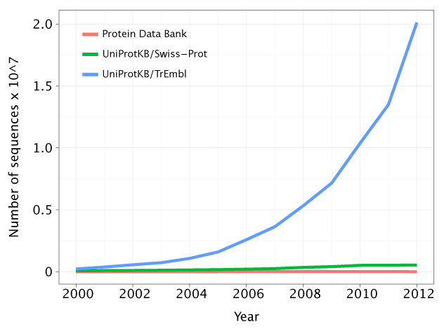
Still, if we look at the number of known genome sequences and known protein structures and at the growth of those figures over the past decade, we look at a drastic scenario:

There is a tendency for the gap between the number of protein sequences and protein structures to increase. Hence, we are getting more and more questions and little to no answers. Observe how the green line (the protein sequences associated with a known or predicted function) is very close to the red line (the number of known protein structures). However, there is a growing gap between the red and the blue line (the number of protein sequences). Source: http://gorbi.irb.hr/en/method/growth-of-sequence-databases/

Well, gathering protein structure data is just as important, if not more important, than gathering sequence data. This motivated the creation of Structural Genomics Consortiums (SGC), facilities that specialize in solving protein structures.

I am sorry to tell you that this is all old news. We have known this for years. Nonetheless, the graph above hasn’t changed. Why? The cost limitations and the experimental difficulties associated with protein structure determination are holding us back. Solving protein structures in the lab is hard and time consuming and we are far from being as efficient at structure determination as we are at genome sequencing.

There is a possible solution to the problem: you start with a protein sequence (a sequential aminoacid list) and you try to predict its structure. This is known as protein structure prediction or protein structure modelling. Well, we have a limited number of building blocks (20) and a good understanding of their physicochemical properties, it shouldn’t be that hard right?

Unfortunately, modelling protein structure is not as simple as calculating how fast a block slides on an inclined plane. Predicting protein structure from sequence is a very hard problem indeed! It has troubled a plethora of minds throughout the past decades, making people lose many nights of sleep (I can vouch for that).

We can attribute that to two major limitations:

1- There are so many possible ways one can combine 20 “blocks” in a sequence of hundreds of aminoacids. Each aminoacid can also assume a limited range of conformations. We are looking at a massive combinatorial problem. The conformational space (the space of valid conformations a protein with a given sequence can assume) is so large that if you could check a single conformation every nanosecond, it would still take longer than the age of the universe to probe all possible conformations.

2- Our physics (and our statistics) are inaccurate. We perform so many approximations in order to make the calculations feasible with current computers that we end up with very inaccurate models.

Ok! So now you should know what protein structure prediction is, why it is important and, more importantly, why it is such a hard problem to solve. I am going to finish off by giving you a brief overview of the two most commons approaches to perform protein structure prediction: template-based modelling (also known as homology modelling) and de novo structure prediction.

There is a general understanding that if two proteins have very similar sequences (namely, if they are homologs), than they will have similar structures. So, we can use known structures of homologs as templates to predict other structures. This is known as homology modelling.

One can do a lot of fancy talk to justify why this works. There is the evolutionary argument: “selective pressure acts on the phenotype level (which can encompass a protein structure) rather than the genotype level. Hence protein structures tend to be more conserved than sequence. For that reason and considering that sequence alone is enough to determine structure, similar sequences will have even more similar structures.”

One can also formulate some sort of physics argument: “a similar aminoacid composition will lead to a similar behaviour of the interacting forces that keep the protein structure packed together. Furthermore, the energy minimum where a certain protein structure sits is so stable that it would take quite a lot of changes in the sequence to disturb that minimum energy conformation drastically.”

Probably the best argument in favour of homology modelling is that it works somewhat well. Of course, the accuracy of the models has a strong dependency on the sequence similarity, but for proteins with more than 40% identity, we can use this method in order to obtain good results.

This raises another issue: what if we can’t find a homolog with known structure? How can we model our templateless protein sequence then? Well, turns out that if we group proteins together into families based on their sequence similarity, more than half of the families would not have a member with known structure. [This data was obtained by looking at the representativeness of the Pfam (a protein family database) on the PDB (a protein structure database).]

Ergo, for a majority of cases we have to perform predictions from scratch (known as free modelling or de novo modelling).

Well, not necessarily from scratch. There is a specific approach to free modelling where we can build our models using existing knowledge. We can use chunks of protein, contiguous fragments extracted from known structures, to generate models. This is known as a fragment-based approach to de novo protein structure prediction. And that is one big name!

One can think of this as a small scale homology modelling, where both the physics and evolutionary arguments should still hold true to some degree. And how do we do? Can we generate good models? We perform appallingly! Accuracies are too low to generate any useful knowledge in a majority of cases. The problem with the rare cases when you get it right is that you have no means to know if you actually got the right answer.

The poor quality of the results can be justified by the 2 biggest limitations discussed above. Yet something else might be in play. In homology modelling, if you use a bad template, you will most certainly get a bad model. In a similar way, using a bad set of fragments will lead you to a very poor final model.

Considering we already have the other two big issues (size of conformational space and accuracy of current potentials) to worry about, we should aim to use the best fragment library we possibly can. This has been the recent focus of my work. An attempt to make a small contribution to solve such a hard problem.

I would love to detail my work on finding better fragments here, but I believe this post is already far too long for anyone to actually endure it and read it until the end. So, congratulations if you made it through!

Journal club: Principles for designing ideal protein structures

The goal of protein design is to generate a sequence that assumes a certain structure and/or performs a specific function. A recent paper in Nature has attempted to design sequences for each of five naturally occurring protein folds. The success rate ranges from 10-40%.

This recent work comes from the Baker group, who are best known for Rosetta and have made several previous steps in this direction. In a 2003 paper this group stripped several naturally occurring proteins down to the backbone, and then generated sequences whose side-chains were consistent with these backbone structures. The sequences were expressed and found to fold into proteins, but the structure of these proteins remained undetermined. Later that same year the group designed a protein, Top7, with a novel fold and confirmed that its structure closely matched that of the design (RMSD of 1.2A).

The proteins designed in these three pieces of work (the current paper and the two papers from 2003) all tend to be more stable than naturally occurring proteins. This increased stability may explain why, as with the earlier Top7, the final structures in the current work closely match the design (RMSD 1 or 2A), despite ab initio structure prediction rarely being this accurate. These structures are designed to sit in a deep potential well in the Rosetta energy function, whereas natural proteins presumably have more complicated energy landscapes that allow for conformational changes and easy degradation. Designing a protein with two or more conformations is a challenge for the future.

In the current work, several sequences were designed for each of the fold types. These sequences have substantial sequence similarity to each other, but do not match existing protein families. The five folds all belong to the alpha + beta or alpha/beta SCOP classes. This is a pragmatic choice: all-alpha proteins often fold into undesired alternative topologies, and all-beta proteins are prone to aggregation. By contrast, rules such as the right-handedness of beta-alpha-beta turns have been known since the 1970s, and can be used to help design a fold.

The authors describe several other rules that influence the packing of beta-alpha-beta, beta-beta-alpha and alpha-beta-beta structural elements. These relate the lengths of the elements and their connective loops with the handedness of the resulting subunit. The rules and their derivations are impressive, but it is not clear to what extent they are applied in the design of the 5 folds. The designed folds contain 13 beta-alpha-beta subunits, but only 2 alpha-beta-beta subunits, and 1 beta-beta-alpha subunit.

An impressive feature of the current work is the use of the Rosetta@home project to select sequences with funnelled energy landscapes, which are less likely to misfold. Each candidate sequence was folded >200000 times from an extended chain. Only ~10% of sequences had a funnelled landscape. It would have been interesting to validate whether the rejected sequences really were less likely to adopt the desired fold — especially given that this selection procedure requires vast computational resources.

The design of these five novel proteins is a great achievement, but even greater challenges remain. The present designs are facilitated by the use of short loops in regions connecting secondary structure elements. Functional proteins will probably require longer loops, more marginal stabilities, and a greater variety of secondary structure subunits.

Talk: Membrane Protein 3D Structure Prediction & Loop Modelling in X-ray Crystallography

Seb gave a talk at the Oxford Structural Genomics Consortium on Wednesday 9 Jan 2013. The talk mentioned the work of several other OPIG members. Below is the gist of it.

Homology modelling pipeline with several membrane-protein-specific steps. Input is the target protein’s sequence, output is the finished 3D model.

Fragment-based loop modelling pipeline for X-ray crystallography

Given an incomplete model of a protein, as well as the current electron density map, we apply our loop modelling method FREAD to fill in a gap with many decoy structures. These decoys are then scored using electron density quality measures computed by EDSTATS. This process can be iterated to arrive at a complete model.

Over the past five years the Oxford Protein Informatics Group has produced several pieces of software to model various aspects of membrane protein structure. iMembrane predicts how a given protein structure sits in the lipid bilayer. MP-T aligns a target protein’s sequence to an iMembrane-annotated template structure. MEDELLER produces an accurate core model of the target, based on this target-template alignment. FREAD then fills in the remaining gaps through fragment-based loop modelling. We have assembled all these pieces of software into a single pipeline, which will be released to the public shortly. In the future, further refinements will be added to account for errors in the core model, such as helix kinks and twists.

X-ray crystallography is the most prevalent way to obtain a protein’s 3D structure. In difficult cases, such as membrane proteins, often only low resolution data can be obtained from such experiments, making the subsequent computational steps to arrive at a complete 3D model that much harder. This usually involves tedious manual building of individual residues and much trial and error. In addition, some regions of the protein (such as disordered loops) simply are not represented by the electron density at all and it is difficult to distinguish these from areas that simply require a lot of work to build. To alleviate some of these problems, we are developing a scoring scheme to attach an absolute quality measure to each residue being built by our loop modelling method FREAD, with a view towards automating protein structure solution at low resolution. This work is being carried out in collaboration with Frank von Delft’s Protein Crystallography group at the Oxford Structural Genomics Consortium.