In last week’s journal club we delved into the history of Ramachandran plots (Half a century of Ramachandran plots; Carugo & Djinovic-Carugo, 2013).

Polypeptide backbone dihedral angles. Source: Wikimedia Commons, Bensaccount

50 years ago Gopalasamudram Narayana Ramachandran et al. predicted the theoretically possible conformations of a polypeptide backbone. The backbone confirmations can be described using three dihedral angles: ω, φ and ψ (shown to the right).

The first angle, ω, is restrained to either about 0° (cis) or about 180° (trans) due to the partial double bond character of the C-N bond. The φ and ψ angles are more interesting, and the Ramachandran plot of a protein is obtained by plotting φ/ψ angles of all residues in a scatter plot.

The original Ramachandran plot showed the allowed conformations of the model compound N-acetyl-L-alanine-methylamide using a hard-sphere atomic model to keep calculations simple. By using two different van der Waals radii for each element positions on the Ramachandran plot could be classified into either allowed regions, regions with moderate clashes and disallowed regions (see Figure 3 (a) in the paper).

The model compound does not take side chains into account, but it does assume that there is a side chain. The resulting Ramachandran plot therefore does not describe the possible φ/ψ angles for Glycine residues, where many more conformations are plausible. On the other end of the spectrum are Proline residues. These have a much more restricted range of possible φ/ψ angles. The φ/ψ distributions of GLY and PRO residues are therefore best described in their own Ramachandran plots (Figure 4 in the paper).

Over time the Ramachandran plot was improved in a number of ways. Instead of relying on theoretical calculations using a model compound, we can now rely on experimental observations by using high quality, hand picked data from the PDB. The way how the Ramachandran plot is calculated has also changed: It can now be seen as a two-dimensional, continuous probability distribution, and can be estimated using a full range of smoothing functions, kernel functions, Fourier series and other models.
The modern Ramachandran plot is much more resolved than the original plot. We now distinguish between a number of well-defined, different regions which correlate with secondary protein structure motifs.

Ramachandran plots are routinely used for structure validation. The inherent circular argument (A good structure does not violate the Ramachandran plot; The plot is obtained by looking at the dihedral angles of good structures) sounds more daring than it actually is. The plot has changed over time, so it is not as self-reinforcing as one might fear. The Ramachandran plot is also not the ultimate guideline. If a new structure is found that claims to violate the Ramachandran plot (which is based on a huge body of cumulative evidence), then this claim needs to be backed up by very good evidence. A low number of violations of the plot can usually be justified. The Ramachandran plot is a local measure. It therefore does not take into account that domains of a protein can exert a force on a few residues and just ‘crunch’ it into an unusual conformation.

The paper closes with a discussion of possible future applications and extensions, such as the distribution of a protein average φ/ψ and an appreciation of modern web-based software and databases that make use of or provide insightful analyses of Ramachandran plots.

In the last journal club we covered the paper Simultaneous Femtosecond X-ray Spectroscopy and Diffraction of Photosystem II at Room Temperature (Kern et al., 2013), currently still in Science Express.

Structure of Photosystem II, PDB 2AXT
CC BY-SA 3.0 Curtis Neveu

This paper describes an experiment on the Photosystem II (PSII) protein complex. PSII is a large protein complex consisting of about 20 subunits with a combined weight of ca. 350 kDa. As its name suggests, this complex plays a crucial role in photosynthesis: it is responsible for the oxidation (“splitting up”) of water.

In the actual experiment (see the top right corner of Figure 1 in the paper) three experimental methods are combined: PSII microcrystals (5-15µm) are injected from the top into the path of an X-ray pulse (blue). Simultaneously, an emission spectrum is recorded (yellow, detector at the bottom). And finally in a separate run the injected crystals are treated (‘pumped’) with a visible laser (red) before they hit the X-ray pulse.

Let’s take a look at each of those three in a little more detail.

X-ray diffraction (XRD)

In a standard macromolecular X-ray crystallography experiment a crystal containing identical molecules of interest (protein) at regular, ordered lattice points is exposed to an X-ray beam. Some X-rays are elastically scattered and cause a diffraction pattern to form on a detector. By analysing the diffraction patterns of a rotating crystal it is possible to calculate the electron density distribution of the molecule in question, and thus determine its three dimensional structure.

An intense X-ray beam however also systematically damages the sample (Garman, 2010). For experiments using in-house X-ray generators or synchrotrons it is therefore recommended not to exceed a total dose of 30 MGy on any one crystal (Owen et al., 2006).

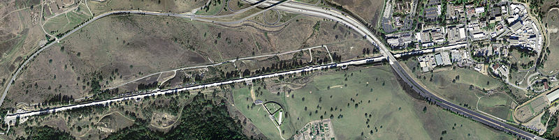
Aerial view of the LCLS site. The accelerator is 3.2 kilometres long.

The experiment described in the current paper however was not conducted using a run-of-the-mill synchrotron, but with the Linac Coherent Light Source (LCLS), an X-ray free electron laser. Here each diffraction image results from an individual crystal exposed to a single X-ray pulse of about 50 femtoseconds, resulting in a peak dose of ~150 MGy. Delivering these extreme doses in very short X-ray pulses lead to the destruction of the sample via a coulomb explosion.

As the sample is destroyed only one diffraction image can be taken per crystal. This causes two complications: Firstly, a large number of sample crystals are required. This explains why the experiment required a total beam time of 6 hours and involved over 2.5 million X-ray shots and processing an equal number of diffraction images. Secondly, the resulting set of (usable) diffraction images are an unordered, random sampling of the crystal orientation space. This presents a computational challenge unique to XFEL setups: before the diffraction data can be integrated, the orientation of the crystal lattice needs to be determined for each individual diffraction image.

X-ray diffraction allows us to obtain a electron density map of the entire unit cell, and therefore the entire crystal. But we can only see ordered areas of the crystal. To really see small molecules in solvent channels, or the conformations of side chains on the protein surface they need to occupy the same positions within each unit cell. For most small molecules this is not the case. This is why you will basically never see compounds like PEGs or Glycerol in your electron density maps, even though you used them during sample preparation. For heavy metal compounds this is especially annoying. They disproportionately increase the X-ray absorption (Holton, 2009; with a handy table 1) and therefore shorten the crystal’s lifetime. But they do not contribute to the diffraction pattern (And that is why you should back-soak; Garman & Murray, 2003).

X-ray emission spectroscopy (XES)

PSII contains a manganese cluster (Mn₄CaO₅). This cluster, as with all protein metallocentres, is known to be highly radiation sensitive (Yano et al., 2005). Apparently at a dose of about 0.75 MGy the cluster is reduced in 50% of the irradiated unit cells.

Diffraction patterns represent a space- and time-average of the electron density. It is very difficult to quantify the amount of reduction from the obtained diffraction patterns. There is however a better and more direct way of measuring the states of the metal atoms: X-ray emission spectroscopy.

Basically the very same events that cause radiation damage also cause X-ray emissions with very specific energies, characteristic for the involved atoms and their oxidation state. An Mn^IVO₂ energy spectrum looks markedly different to an Mn^IIO spectrum (bottom right corner of Figure 1).

The measurements of XRD and XES are taken simultaneously. But, differently to XRD, XES does not rely on crystalline order. It makes no difference whether the metallocentres move within the unit cell as a result of specific radiation damage. Even the destruction of the sample is not an issue: we can assume that XES will record the state of the clusters regardless of the state of the crystal lattice – up to the point where the whole sample blows up. But at that point we know that due to the loss of long-range order the X-ray diffraction pattern will no longer be affected.

The measurements of XES therefore give us a worst-case scenario of the state of the manganese cluster in the time-frame where we obtained the X-ray diffraction data.

Induced protein state transition with visible laser

Another neat technique used in this experiment is the activation of the protein by a visible laser in the flight path of the crystals as they approach the X-ray interaction zone. With a known crystal injection speed and a known distance between the visible laser and the X-ray pulse it becomes possible to observe time-dependent protein processes (top left corner of Figure 1).

What makes this paper special? (And why is it important to my work?)

It has been theorized and partially known that the collection of diffraction data using X-ray free electron lasers outruns traditional radiation damage processes. Yet there was no conclusive proof – up until now.

This paper has shown that the XES spectra of the highly sensitive metallocentres do not indicate any measurable (let alone significant) change from the idealized intact state (Figure 3). Apparently the highly sensitive metallocentres of the protein stay intact up to the point of complete sample destruction, and certainly well beyond the point of sample diffraction.

Or to put another way: even though the crystalline sample itself is destroyed under extreme conditions, the obtained diffraction pattern is – for all intents and purposes – that of an intact, pristine, zero dose state of the crystal.

This is an intriguing result for people interested in macromolecular crystallography radiation damage. In a regime of absurdly high doses, where the entire concept of a ‘dose’ for a crystal breaks down (again), we can obtain structural data with no specific radiation damage present at the metallocentres. As metallocentres are more susceptible to specific radiation damage it stands to reason that the diffraction data may be free of all specific damage artefacts.

It is thought that most deposited PDB protein structures containing metallocentres are in a reduced state. XFELs are being constructed all over the world and will be the next big thing in macromolecular crystallography. And now it seems that the future of metalloproteins got even brighter.